Vicsek dynamics, order-disorder transitions, and agent-based rules
Local Rules, Global Order
Collective motion is the first session where the main model is not a continuous-time ODE. The dynamics come from a repeated update rule applied to many agents at once.
Session Arc
Base rule
Start with Vicsek alignment, noise, constant speed, and periodic boundaries.
Observable
Measure the transition with the order parameter instead of relying on animation alone.
Extensions
Then ask what changes when you add repulsion, predators, or richer decision rules.
Why This Is Not an ODE Session
Previous sessions
State changes came from derivatives and continuous-time rate laws.
This session
Each time step updates headings and positions directly from neighbor information, so a simulation loop is more natural than solve_ivp().
At each step, every boid aligns with neighbors inside a radius \(r\), adds noise, moves at constant speed, and wraps back into the box with periodic boundary conditions.
What Moves the Transition
Noise \(\eta\)
Higher noise breaks alignment and pushes the system toward disorder.
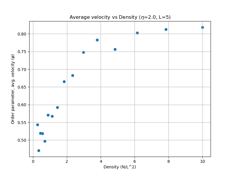
Density
More local contacts make alignment easier.
Interaction radius \(r\)
This sets who can influence whom at each step.
Speed \(v_0\)
This controls how quickly local alignment propagates through the box.
The Order Parameter Is the Summary Statistic
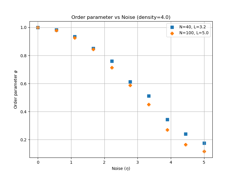
Order parameter versus noise
Average velocity versus density
Use the average normalized velocity to quantify how ordered the flock is. The interesting part is the transition, not just the animation.
The Session Extends in Two Directions
Couzin model
Add a repulsion zone so agents avoid collisions instead of only aligning.
Predator extension
Add an escape rule, then decide whether the predator is passive, autonomous, or includes eating-spawning dynamics.