Before animating the Vicsek model, it is important to validate your implementation and build intuition about how the parameters affect collective motion (Vicsek et al. 1995). Here, you will use static plots to explore how the interaction radius \(r\) influences the alignment of particles. This step helps ensure your code is working as expected and provides insight into the model’s behavior before moving on to more complex analyses or animations.
We will run the Vicsek model for a few time steps and visualize the headings of all particles for different values of \(r\). This will help you see the transition from random motion to local and global alignment as the interaction radius increases.
Follow the structure below:
import matplotlib.pyplot as plt# Initialize parametersnum_particles =100box_size =10# Linteraction_radius =1.0# rnoise_strength =0.1# etav0 =0.03# speed of particles# Initialize particle positions and headingsxy, theta = initialize_particles(num_particles, box_size)# Update positions and headings for a few time stepsfor t inrange(10): xy, theta = vicsek_equations( xy=xy, theta=theta, noise=noise_strength, box_size=box_size, radius_interaction=interaction_radius, v0=v0, )# Plot the headings of the particlesplt.figure(figsize=(6, 6))plt.quiver( xy[0], xy[1], np.cos(theta), np.sin(theta), angles='xy', scale_units='xy', scale=2, # bigger scale means smaller arrows)# Limit the plot to the box sizeplt.xlim(0, box_size)plt.ylim(0, box_size)plt.title('Particle headings after 10 time steps')plt.xlabel('x')plt.ylabel('y')plt.grid()plt.show()
Run the code above with three interaction radii: \(r = 0\), \(r = L / 10\), and \(r = L\), where \(L\) is the box size. What do you observe? How does the interaction radius affect the alignment of the particles?
Answer for \(r = 0\)
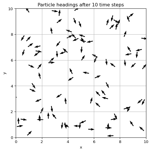
For \(r = 0\), there is no interaction between particles, so they will move in random directions based on their initial headings and noise. The plot will show a random distribution of arrows with no clear alignment.
Particle headings for \(r = 0\)
Answer for \(r = L / 10\)
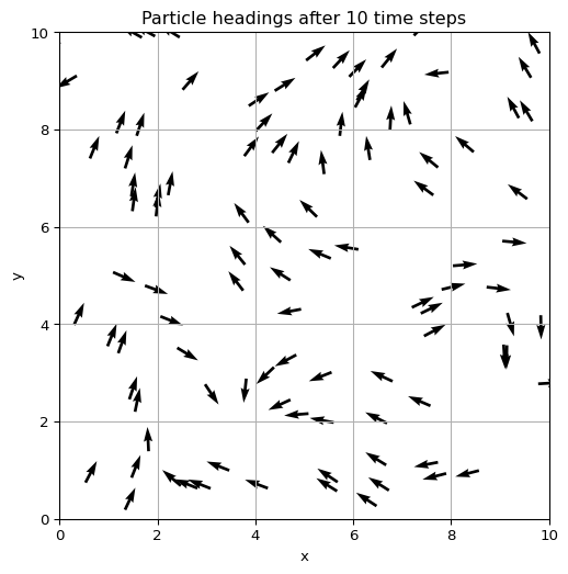
For \(r = L / 10\), particles will interact with others within a radius of one-tenth of the box size. This means that each particle will have a limited chance to align with nearby particles, leading to small local clusters of aligned particles. The plot will show groups of arrows pointing in similar directions, indicating partial alignment.
Particle headings for \(r = L / 10\)
Answer for \(r = L\)
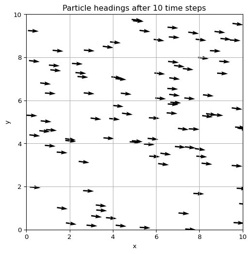
For \(r = L\), particles will interact with all other particles in the box. This means that each particle will tend to align with the average direction of all particles, leading to global alignment. The plot will show arrows mostly pointing in the same direction, indicating strong alignment.
Particle headings for \(r = L\)
References
Vicsek, Tamás, András Czirók, Eshel Ben-Jacob, Inon Cohen, and Ofer Shochet. 1995. “Novel Type of Phase Transition in a System of Self-Driven Particles.”Physical Review Letters 75 (6): 1226.
Source Code
---title: "Vicsek Model: Validation"subtitle: "Static Analysis of Collective Motion"format: html---Before animating the Vicsek model, it is important to validate your implementation and build intuition about how the parameters affect collective motion [@vicsek1995novel]. Here, you will use static plots to explore how the interaction radius $r$ influences the alignment of particles. This step helps ensure your code is working as expected and provides insight into the model's behavior before moving on to more complex analyses or animations.We will run the Vicsek model for a few time steps and visualize the headings of all particles for different values of $r$. This will help you see the transition from random motion to local and global alignment as the interaction radius increases.Follow the structure below:```pythonimport matplotlib.pyplot as plt# Initialize parametersnum_particles =100box_size =10# Linteraction_radius =1.0# rnoise_strength =0.1# etav0 =0.03# speed of particles# Initialize particle positions and headingsxy, theta = initialize_particles(num_particles, box_size)# Update positions and headings for a few time stepsfor t inrange(10): xy, theta = vicsek_equations( xy=xy, theta=theta, noise=noise_strength, box_size=box_size, radius_interaction=interaction_radius, v0=v0, )# Plot the headings of the particlesplt.figure(figsize=(6, 6))plt.quiver( xy[0], xy[1], np.cos(theta), np.sin(theta), angles='xy', scale_units='xy', scale=2, # bigger scale means smaller arrows)# Limit the plot to the box sizeplt.xlim(0, box_size)plt.ylim(0, box_size)plt.title('Particle headings after 10 time steps')plt.xlabel('x')plt.ylabel('y')plt.grid()plt.show()```Run the code above with three interaction radii: $r = 0$, $r = L / 10$, and $r = L$, where $L$ is the box size. What do you observe? How does the interaction radius affect the alignment of the particles?::: {.callout-tip collapse="true"}## Answer for $r = 0$For $r = 0$, there is no interaction between particles, so they will move in random directions based on their initial headings and noise. The plot will show a random distribution of arrows with no clear alignment.```{python}#| label: answer-r-0#| echo: false#| fig-cap: "Particle headings for $r = 0$"#| fig-width: 6#| fig-height: 6import numpy as npimport matplotlib.pyplot as pltfrom amlab.collective_motion.vicsek import initialize_particles, vicsek_equations# Initialize parametersnum_particles =100box_size =10# Linteraction_radius =0# rnoise_strength =0.1# etav0 =0.03# speed of particles# Initialize particle positions and headingsxy, theta = initialize_particles(num_particles, box_size)# Update positions and headings for a few time stepsfor t inrange(10): xy, theta = vicsek_equations( xy=xy, theta=theta, noise=noise_strength, box_size=box_size, radius_interaction=interaction_radius, v0=v0, )# Plot the headings of the particlesplt.figure(figsize=(6, 6))plt.quiver( xy[0], xy[1], np.cos(theta), np.sin(theta), angles='xy', scale_units='xy', scale=2,)# Limit the plot to the box sizeplt.xlim(0, box_size)plt.ylim(0, box_size)plt.title('Particle headings after 10 time steps')plt.xlabel('x')plt.ylabel('y')plt.grid()plt.show()```:::::: {.callout-tip collapse="true"}## Answer for $r = L / 10$For $r = L / 10$, particles will interact with others within a radius of one-tenth of the box size. This means that each particle will have a limited chance to align with nearby particles, leading to small local clusters of aligned particles. The plot will show groups of arrows pointing in similar directions, indicating partial alignment.```{python}#| label: answer-r-l10#| echo: false#| fig-cap: "Particle headings for $r = L / 10$"#| fig-width: 6#| fig-height: 6import numpy as npimport matplotlib.pyplot as pltfrom amlab.collective_motion.vicsek import initialize_particles, vicsek_equations# Initialize parametersnum_particles =100box_size =10# Linteraction_radius = box_size /10# rnoise_strength =0.1# etav0 =0.03# speed of particles# Initialize particle positions and headingsxy, theta = initialize_particles(num_particles, box_size)# Update positions and headings for a few time stepsfor t inrange(10): xy, theta = vicsek_equations( xy=xy, theta=theta, noise=noise_strength, box_size=box_size, radius_interaction=interaction_radius, v0=v0, )# Plot the headings of the particlesplt.figure(figsize=(6, 6))plt.quiver( xy[0], xy[1], np.cos(theta), np.sin(theta), angles='xy', scale_units='xy', scale=2,)# Limit the plot to the box sizeplt.xlim(0, box_size)plt.ylim(0, box_size)plt.title('Particle headings after 10 time steps')plt.xlabel('x')plt.ylabel('y')plt.grid()plt.show()```:::::: {.callout-tip collapse="true"}## Answer for $r = L$For $r = L$, particles will interact with all other particles in the box. This means that each particle will tend to align with the average direction of all particles, leading to global alignment. The plot will show arrows mostly pointing in the same direction, indicating strong alignment.```{python}#| label: answer-r-l#| echo: false#| fig-cap: "Particle headings for $r = L$"#| fig-width: 6#| fig-height: 6import numpy as npimport matplotlib.pyplot as pltfrom amlab.collective_motion.vicsek import initialize_particles, vicsek_equations# Initialize parametersnum_particles =100box_size =10# Linteraction_radius = box_size # rnoise_strength =0.1# etav0 =0.03# speed of particles# Initialize particle positions and headingsxy, theta = initialize_particles(num_particles, box_size)# Update positions and headings for a few time stepsfor t inrange(10): xy, theta = vicsek_equations( xy=xy, theta=theta, noise=noise_strength, box_size=box_size, radius_interaction=interaction_radius, v0=v0, )# Plot the headings of the particlesplt.figure(figsize=(6, 6))plt.quiver( xy[0], xy[1], np.cos(theta), np.sin(theta), angles='xy', scale_units='xy', scale=2,)# Limit the plot to the box sizeplt.xlim(0, box_size)plt.ylim(0, box_size)plt.title('Particle headings after 10 time steps')plt.xlabel('x')plt.ylabel('y')plt.grid()plt.show()```:::