SIS Model

Susceptible-Infected-Susceptible

In the SIS model, infected nodes recover back to susceptible. At each step:

• A susceptible node becomes infected with probability \(\beta\) for each infected neighbor.
• An infected node recovers with probability \(\gamma\).

Figure 1: SIS model: example network with one infected node.

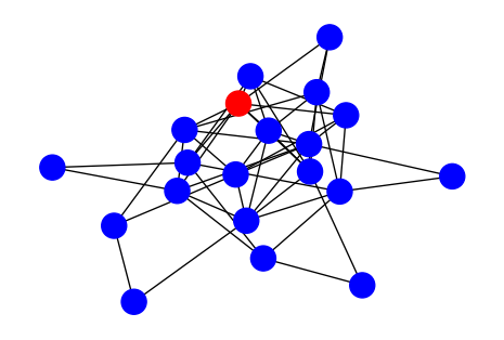
Step 1: Initialize the graph

Choose a network structure and draw it.

import networkx as nx
import matplotlib.pyplot as plt

G = nx.gnm_random_graph(n=20, m=50)
pos = nx.spring_layout(G)

nx.draw(G, pos)
plt.show()

Step 2: Add a node state

Each node has a state: “S” or “I”. Start with one infected node.

node_names = list(G.nodes)
state = {}
# TODO: set one node to "I" and the rest to "S"

nx.set_node_attributes(G, state, "state")

Hint: Initial state (click to expand)

state = {node: "S" for node in G.nodes}
patient_zero = node_names[0]
state[patient_zero] = "I"

Step 3: State transition

Implement the SIS transition rules.

state = nx.get_node_attributes(G, "state")
next_state = {}

# TODO: implement SIS transitions using beta and gamma

nx.set_node_attributes(G, next_state, "state")

Hint: SIS transition (click to expand)

import random

next_state = {}
for node in G.nodes:
    if state[node] == "I":
        if random.random() < gamma:
            next_state[node] = "S"
    else:
        for neighbor in G.neighbors(node):
            if state[neighbor] == "I" and random.random() < beta:
                next_state[node] = "I"
                break

Step 4: Simulate and plot

Run for multiple steps and track the number of S and I nodes.

num_steps = 100
ls_s, ls_i = [], []

for _ in range(num_steps):
    # TODO: apply the transition and update attributes
    counts = list(nx.get_node_attributes(G, "state").values())
    ls_s.append(counts.count("S"))
    ls_i.append(counts.count("I"))

# TODO: plot ls_s and ls_i

Extra challenge

Extend the model to SIR or SIRS by adding a recovered state.

If you want a full reference, see amlab/networks_complex/simulation.py.