Turing Instability

From Steady States to Spatial Modes

In the previous page, you built a 1D reaction-diffusion solver and saw that small perturbations can grow into visible peaks. This page explains when that should happen.

Patterns do not appear by accident. Turing instability explains when a uniform steady state is stable to homogeneous perturbations but unstable to spatially varying ones (Turing 1952). For the Gierer-Meinhardt model, the same theory will help us interpret both the 1D and 2D simulations.

The previous page gave the intuition: local activation can reinforce a bump, inhibition can suppress nearby growth, and diffusion can either smooth or amplify spatial differences depending on the parameter regime. This page turns that picture into a linear stability test and asks a precise question, which parameter values and which spatial modes make the flat steady state lose stability?

Figure 1: Turing space for the Gierer-Meinhardt model in the \((a, d)\) plane.

The Linear Stability Pipeline

For a two-species reaction-diffusion system

\[ \partial_t w = D\,\Delta w + R(w), \qquad D = \operatorname{diag}(d_1, d_2), \]

start from a homogeneous steady state \(w_*\) with \(R(w_*) = 0\). Write \(w = w_* + \eta\) and keep only linear terms:

\[ \partial_t \eta = D\,\Delta \eta + J\eta, \]

where

\[ J = \begin{pmatrix} f_u & f_v \\ g_u & g_v \end{pmatrix} \tag{1}\]

is the Jacobian of the reaction terms at the steady state.

Now expand the perturbation in Laplacian eigenmodes,

\[ \eta(x,t) = c_n(t)\,\phi_n(x), \qquad \Delta \phi_n = \lambda_n \phi_n, \qquad \lambda_n \le 0. \]

Each spatial mode evolves independently as

\[ \dot c_n = F_n c_n, \qquad F_n = J + \lambda_n D. \tag{2}\]

Because \(\lambda_n = -k_n^2\), many notes write the same matrix as

\[ A_n = J - k_n^2 D. \tag{3}\]

So the workflow is always the same.

Find the homogeneous equilibrium.
Compute the Jacobian at that equilibrium.
Compute the Laplacian eigenvalues \(\lambda_n\) from the domain and the boundary conditions.
Build \(F_n\) or \(A_n\).
Compute the eigenvalues of that \(2 \times 2\) matrix.
Keep the modes whose largest real part is positive.

For a \(2 \times 2\) matrix, the growth rates \(\sigma\) satisfy

\[ \sigma^2 - \operatorname{tr}(F_n)\sigma + \det(F_n) = 0. \]

With \(D = \operatorname{diag}(1, d)\), the diffusion-shifted matrix has

\[ \operatorname{tr}(A_n) = (f_u + g_v) - (1 + d)k_n^2, \]

\[ \det(A_n) = (f_u g_v - f_v g_u) - (d f_u + g_v)k_n^2 + d k_n^4. \tag{4}\]

Diffusion makes the trace more negative, so the Turing mechanism is detected through the determinant. The flat state is stable when \(\operatorname{tr}(J) < 0\) and \(\det(J) > 0\). A Turing instability appears when some nonzero mode makes \(\det(A_n) < 0\).

Compute the Gierer-Meinhardt Equilibrium

For the Gierer-Meinhardt model,

\[ f(u, v) = a - b u + \frac{u^2}{v}, \qquad g(u, v) = u^2 - v. \]

The homogeneous steady state solves \(f(u_*, v_*) = 0\) and \(g(u_*, v_*) = 0\). From \(g(u_*, v_*) = 0\) we get \(v_* = u_*^2\). Substituting into \(f = 0\) gives

\[ u_* = \frac{a+1}{b}, \qquad v_* = \left(\frac{a+1}{b}\right)^2. \tag{5}\]

def gierer_meinhardt_equilibrium(a=0.40, b=1.00):
    u_star = (a + 1) / b
    v_star = u_star**2
    return u_star, v_star

Write the Jacobian at the Fixed Point

At a general point \((u, v)\), the Jacobian is

\[ J(u, v) = \begin{pmatrix} -b + 2u/v & -u^2/v^2 \\ 2u & -1 \end{pmatrix}. \]

Evaluating at \((u_*, v_*)\) gives the entries needed for the Turing test.

def gierer_meinhardt_jacobian(a=0.40, b=1.00):
    u_star, v_star = gierer_meinhardt_equilibrium(a, b)
    fu = -b + 2 * u_star / v_star
    fv = -(u_star**2) / (v_star**2)
    gu = 2 * u_star
    gv = -1.0
    return fu, fv, gu, gv

Hint: Jacobian entries (click to expand)

def gierer_meinhardt_jacobian(a=0.40, b=1.00):
    fu = 2 * b / (a + 1) - b
    fv = -((b / (a + 1)) ** 2)
    gu = 2 * (a + 1) / b
    gv = -1.0
    return fu, fv, gu, gv

Implement the Turing Test

From \(\operatorname{tr}(J) < 0\), \(\det(J) > 0\), and the requirement that \(\det(A_n)\) becomes negative for some nonzero mode, we recover the standard three conditions

\[ \begin{aligned} &f_u + g_v < 0, \\ &f_u g_v - f_v g_u > 0, \\ &g_v + d f_u > 2\sqrt{d\,(f_u g_v - f_v g_u)}. \end{aligned} \tag{6}\]

The last inequality is exactly the statement that the quadratic \(\det(A_n)\) dips below zero for some \(k_n^2 > 0\).

Translate these three inequalities into Python.

import numpy as np

def is_turing_instability(a, b, d):
    fu, fv, gu, gv = gierer_meinhardt_jacobian(a, b)
    nabla =

    # TODO: write the three conditions
    cond1 =
    cond2 =
    cond3 =
    return cond1 & cond2 & cond3

Hint: Turing test (click to expand)

def is_turing_instability(a, b, d):
    fu, fv, gu, gv = gierer_meinhardt_jacobian(a, b)
    nabla = fu * gv - fv * gu
    cond1 = (fu + gv) < 0
    cond2 = nabla > 0
    cond3 = (gv + d * fu) > 2 * np.sqrt(d * np.maximum(nabla, 0))
    return cond1 & cond2 & cond3

If your implementation is vectorized, it should work with scalars and with arrays. That is what lets us plot Figure 1.

Validate these functions carefully. You will reuse them when you move from 1D to 2D, so this is the theory page that supports the rest of the session.

Plot the Turing Space

Complete the code below to recreate the diagram.

import matplotlib.pyplot as plt
import numpy as np

arr_a = np.linspace(0, 1, 500)
arr_d = np.linspace(0, 100, 500)
mesh_a, mesh_d = np.meshgrid(arr_a, arr_d)
mask_turing =

fig, ax = plt.subplots(figsize=(7, 4))
ax.contourf(mesh_a, mesh_d, mask_turing)
ax.set_xlabel("a")
ax.set_ylabel("d")
ax.set_title("Turing Space")
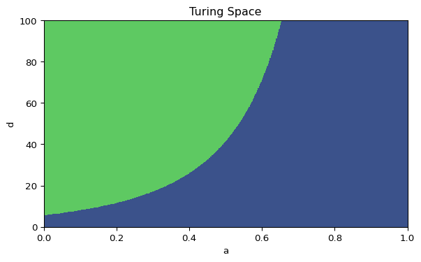
plt.show()

Mark the point \((a, d) = (0.40, 20)\) on your plot. Is it inside the instability region?

This is the same Turing-space diagram that appears in the left panel of the interactive Gierer-Meinhardt code, so the algebra and the simulation refer to the same parameter plane.

Compute \(F_n\) and the Unstable Mode List in 1D

The Turing conditions say that some spatial mode should grow, but they do not tell you which one. For Neumann boundary conditions on \([0, L]\), the Laplacian eigenvalues are

\[ \lambda_n = -\left(\frac{n\pi}{L}\right)^2, \qquad n = 0, 1, 2, \dots \tag{7}\]

Equivalently, \(k_n = n\pi/L\). The mode matrix is

\[ F_n = J + \lambda_n\,\mathrm{diag}(1, d) = J - k_n^2\,\mathrm{diag}(1, d). \tag{8}\]

Compute the eigenvalues of each \(F_n\), keep the modes with positive growth, and sort them from strongest to weakest.

import numpy as np

def find_unstable_modes_1d(a=0.40, b=1.00, d=30.0, length=40.0, num_modes=10):
    fu, fv, gu, gv = gierer_meinhardt_jacobian(a, b)
    jac = np.array([[fu, fv], [gu, gv]])
    diffusion = np.diag([1.0, d])
    unstable_modes = []

    for n in range(1, num_modes):
        # TODO: compute lambda_n and the matrix F_n
        # TODO: store modes with positive largest real part

    # TODO: return the unstable modes sorted from strongest to weakest

Hint: 1D mode scan (click to expand)

def find_unstable_modes_1d(a=0.40, b=1.00, d=30.0, length=40.0, num_modes=10):
    fu, fv, gu, gv = gierer_meinhardt_jacobian(a, b)
    jac = np.array([[fu, fv], [gu, gv]])
    diffusion = np.diag([1.0, d])
    unstable_modes = []

    for n in range(1, num_modes):
        lambda_n = -(n * np.pi / length) ** 2
        f_n = jac + lambda_n * diffusion
        growth_rate = np.max(np.linalg.eigvals(f_n).real)
        if growth_rate > 0:
            unstable_modes.append((n, growth_rate))

    unstable_modes.sort(key=lambda item: item[1], reverse=True)
    return unstable_modes

The first entry in this list is the dominant linear mode, which predicts the earliest visible wavelength in the simulation.

Extend the Scan to 2D

In two dimensions, the modes are pairs \((n_x, n_y)\). On a rectangle with side lengths \(L_x\) and \(L_y\) and Neumann boundaries,

\[ \lambda_{n_x,n_y} = -\left(\frac{n_x\pi}{L_x}\right)^2 - \left(\frac{n_y\pi}{L_y}\right)^2. \tag{9}\]

The only real change is that you now scan a grid of mode pairs and build

\[ F_{n_x,n_y} = J + \lambda_{n_x,n_y}\,\mathrm{diag}(1, d). \]

import numpy as np

def find_unstable_modes_2d(a=0.40, b=1.00, d=30.0, length_x=20.0, length_y=50.0, num_modes=8):
    fu, fv, gu, gv = gierer_meinhardt_jacobian(a, b)
    jac = np.array([[fu, fv], [gu, gv]])
    diffusion = np.diag([1.0, d])
    unstable_modes = []

    for nx in range(num_modes):
        for ny in range(num_modes):
            if nx == 0 and ny == 0:
                continue

            # TODO: compute lambda_nm and F_nm
            # TODO: store mode pairs with positive growth rate

    return unstable_modes

::: {.callout-tip collapse=“true”} ## Hint: 2D mode scan (click to expand)

def find_unstable_modes_2d(a=0.40, b=1.00, d=30.0, length_x=20.0, length_y=50.0, num_modes=8):
    fu, fv, gu, gv = gierer_meinhardt_jacobian(a, b)
    jac = np.array([[fu, fv], [gu, gv]])
    diffusion = np.diag([1.0, d])
    unstable_modes = []

    for nx in range(num_modes):
        for ny in range(num_modes):
            if nx == 0 and ny == 0:
                continue

            lambda_nm = -((nx * np.pi / length_x) ** 2 + (ny * np.pi / length_y) ** 2)
            f_nm = jac + lambda_nm * diffusion
            growth_rate = np.max(np.linalg.eigvals(f_nm).real)
            if growth_rate > 0:
                unstable_modes.append(((nx, ny), growth_rate))

    unstable_modes.sort(key=lambda item: item[1], reverse=True)
    return unstable_modes

For periodic boundaries, the same loop works after replacing each factor of $\pi / L$ by $2\pi / L$.

## Apply the Same Workflow to Gray-Scott

The theory on this page does not depend on the specific reaction law. Gray-Scott uses the same equilibrium to Jacobian to mode-matrix pipeline [@gray1984autocatalytic; @pearson1993complex].

Write the reaction terms as

$$
R_u(u, v) = -u v^2 + f(1-u), \qquad R_v(u, v) = u v^2 - (f+k)v.
$$

One homogeneous equilibrium is always

$$
(u_*, v_*) = (1, 0).
$$

If $v_* \neq 0$, then $u_* v_* = f + k$ and the nontrivial equilibria satisfy

$$
u_* = \frac{1}{2}\left(1 \pm \sqrt{1 - \frac{4(f+k)^2}{f}}\right), \qquad v_* = \frac{f+k}{u_*},
$$ {#eq-pde-turing-gs-steady}

whenever $1 - 4(f+k)^2/f \ge 0$.

The Gray-Scott Jacobian at a homogeneous equilibrium is

$$
J_{\mathrm{GS}} =
\begin{pmatrix}
-v_*^2 - f & -2u_*v_* \\
v_*^2 & 2u_*v_* - (f+k)
\end{pmatrix}.
$$ {#eq-pde-turing-gs-jacobian}

At the trivial state $(1, 0)$, this Jacobian is diagonal and every linear mode decays. So the classical Turing test is only interesting at a nontrivial homogeneous equilibrium when one exists.

For periodic boundaries on a rectangle,

$$
\lambda_{m,n} = -\left(\frac{2\pi m}{L_x}\right)^2 - \left(\frac{2\pi n}{L_y}\right)^2,
$$

and the mode matrix is

$$
F^{\mathrm{GS}}_{m,n} = J_{\mathrm{GS}} + \lambda_{m,n}\,\mathrm{diag}(d_1, d_2).
$$

```python
import numpy as np

def gray_scott_equilibria(f=0.040, k=0.060):
    equilibria = [(1.0, 0.0)]
    discriminant = 1 - 4 * (f + k) ** 2 / f

    if discriminant >= 0:
        root = np.sqrt(discriminant)
        for sign in (+1, -1):
            u_star = 0.5 * (1 + sign * root)
            if u_star > 0:
                equilibria.append((u_star, (f + k) / u_star))

    return equilibria


def gray_scott_jacobian(u_star, v_star, f=0.040, k=0.060):
    return np.array(
        [
            [-v_star**2 - f, -2 * u_star * v_star],
            [v_star**2, 2 * u_star * v_star - (f + k)],
        ]
    )

That is the whole bridge from Gierer-Meinhardt to Gray-Scott. Keep the eigenvalue scan, replace the Jacobian, replace the boundary spectrum, then sort the unstable modes and read off the dominant one.

:::

## Compare Two Cases

Use your functions to compare $d=20$ and $d=30$ with $a=0.40$ and $b=1.00$.

1. Does each case satisfy the Turing conditions?
2. How many unstable modes appear in 1D?
3. What is the leading mode in 2D?

These answers will help you interpret the 1D assignment now and the 2D simulations in the next session.

## What's Next?

Now that you know how to predict pattern-forming parameter regimes, close the 1D loop by completing the assignment. After that, carry the same ideas to a 2D grid in the next session.

[Assignment](assignment.qmd){.btn .btn-secondary}
[PDEs in 2D](../pde-2d/index.qmd){.btn .btn-primary}

::: {.callout-tip}
Reference code is available in [amlab/pdes/gierer_meinhardt_1d.py](https://github.com/daniprec/BAM-Applied-Math-Lab/blob/main/amlab/pdes/gierer_meinhardt_1d.py) and [amlab/pdes/gierer_meinhardt_2d.py](https://github.com/daniprec/BAM-Applied-Math-Lab/blob/main/amlab/pdes/gierer_meinhardt_2d.py).
:::





:::{#quarto-navigation-envelope .hidden}
[Applied Math Lab]{.hidden render-id="quarto-int-sidebar-title"}
[Applied Math Lab]{.hidden render-id="quarto-int-navbar-title"}
[Assignment]{.hidden render-id="quarto-int-next"}
[Gierer-Meinhardt 1D]{.hidden render-id="quarto-int-prev"}
[Getting Started]{.hidden render-id="quarto-int-sidebar:quarto-sidebar-section-1"}
[Home]{.hidden render-id="quarto-int-sidebar:/index.htmlHome"}
[Syllabus]{.hidden render-id="quarto-int-sidebar:/syllabus.htmlSyllabus"}
[ODEs in 1D]{.hidden render-id="quarto-int-sidebar:quarto-sidebar-section-2"}
[SIR Epidemic Model]{.hidden render-id="quarto-int-sidebar:/modules/ode-1d/sir.htmlSIR-Epidemic-Model"}
[Michaelis–Menten Kinetics]{.hidden render-id="quarto-int-sidebar:/modules/ode-1d/michaelis-menten.htmlMichaelis–Menten-Kinetics"}
[Spruce Budworm Model]{.hidden render-id="quarto-int-sidebar:/modules/ode-1d/spruce-budworm.htmlSpruce-Budworm-Model"}
[Assignment]{.hidden render-id="quarto-int-sidebar:/modules/ode-1d/assignment.htmlAssignment"}
[ODEs in 2D]{.hidden render-id="quarto-int-sidebar:quarto-sidebar-section-3"}
[CDIMA Reaction]{.hidden render-id="quarto-int-sidebar:/modules/ode-2d/cdima.htmlCDIMA-Reaction"}
[Van der Pol Oscillator]{.hidden render-id="quarto-int-sidebar:/modules/ode-2d/van-der-pol.htmlVan-der-Pol-Oscillator"}
[FitzHugh–Nagumo Model]{.hidden render-id="quarto-int-sidebar:/modules/ode-2d/fitzhugh-nagumo.htmlFitzHugh–Nagumo-Model"}
[Animation Template]{.hidden render-id="quarto-int-sidebar:/modules/ode-2d/animation.htmlAnimation-Template"}
[Assignment]{.hidden render-id="quarto-int-sidebar:/modules/ode-2d/assignment.htmlAssignment"}
[Coupled ODEs]{.hidden render-id="quarto-int-sidebar:quarto-sidebar-section-4"}
[Kuramoto Model]{.hidden render-id="quarto-int-sidebar:/modules/ode-coupled/kuramoto.htmlKuramoto-Model"}
[Kuramoto: Oscillators]{.hidden render-id="quarto-int-sidebar:/modules/ode-coupled/kuramoto-oscillators.htmlKuramoto:-Oscillators"}
[Kuramoto: Bifurcation Diagram]{.hidden render-id="quarto-int-sidebar:/modules/ode-coupled/kuramoto-diagram.htmlKuramoto:-Bifurcation-Diagram"}
[Kuramoto: Full Simulation]{.hidden render-id="quarto-int-sidebar:/modules/ode-coupled/kuramoto-full.htmlKuramoto:-Full-Simulation"}
[Assignment]{.hidden render-id="quarto-int-sidebar:/modules/ode-coupled/assignment.htmlAssignment"}
[Collective Motion]{.hidden render-id="quarto-int-sidebar:quarto-sidebar-section-5"}
[Vicsek Model]{.hidden render-id="quarto-int-sidebar:/modules/collective-motion/vicsek.htmlVicsek-Model"}
[Vicsek Validation]{.hidden render-id="quarto-int-sidebar:/modules/collective-motion/vicsek-validation.htmlVicsek-Validation"}
[Vicsek Animation]{.hidden render-id="quarto-int-sidebar:/modules/collective-motion/vicsek-animation.htmlVicsek-Animation"}
[Vicsek Animation (Interactive)]{.hidden render-id="quarto-int-sidebar:/modules/collective-motion/vicsek-animation-interactive.htmlVicsek-Animation-(Interactive)"}
[Couzin Model]{.hidden render-id="quarto-int-sidebar:/modules/collective-motion/couzin.htmlCouzin-Model"}
[Vicsek with Predator]{.hidden render-id="quarto-int-sidebar:/modules/collective-motion/vicsek-predator.htmlVicsek-with-Predator"}
[Assignment]{.hidden render-id="quarto-int-sidebar:/modules/collective-motion/assignment.htmlAssignment"}
[Networks]{.hidden render-id="quarto-int-sidebar:quarto-sidebar-section-6"}
[Network Fundamentals]{.hidden render-id="quarto-int-sidebar:/modules/networks/fundamentals.htmlNetwork-Fundamentals"}
[Network Connectivity]{.hidden render-id="quarto-int-sidebar:/modules/networks/connectivity.htmlNetwork-Connectivity"}
[Graph Models]{.hidden render-id="quarto-int-sidebar:/modules/networks/models.htmlGraph-Models"}
[SIS Model]{.hidden render-id="quarto-int-sidebar:/modules/networks/sis.htmlSIS-Model"}
[SIR Model]{.hidden render-id="quarto-int-sidebar:/modules/networks/sir.htmlSIR-Model"}
[Assignment]{.hidden render-id="quarto-int-sidebar:/modules/networks/assignment.htmlAssignment"}
[PDEs in 1D]{.hidden render-id="quarto-int-sidebar:quarto-sidebar-section-7"}
[Gierer-Meinhardt 1D]{.hidden render-id="quarto-int-sidebar:/modules/pde-1d/gierer-meinhardt-1d.htmlGierer-Meinhardt-1D"}
[Turing Instability]{.hidden render-id="quarto-int-sidebar:/modules/pde-1d/turing-instability.htmlTuring-Instability"}
[Assignment]{.hidden render-id="quarto-int-sidebar:/modules/pde-1d/assignment.htmlAssignment"}
[PDEs in 2D]{.hidden render-id="quarto-int-sidebar:quarto-sidebar-section-8"}
[Gierer-Meinhardt 2D]{.hidden render-id="quarto-int-sidebar:/modules/pde-2d/gierer-meinhardt-2d.htmlGierer-Meinhardt-2D"}
[Gray-Scott]{.hidden render-id="quarto-int-sidebar:/modules/pde-2d/gray-scott.htmlGray-Scott"}
[Gray-Scott: Interaction]{.hidden render-id="quarto-int-sidebar:/modules/pde-2d/gray-scott-art.htmlGray-Scott:-Interaction"}
[Assignment]{.hidden render-id="quarto-int-sidebar:/modules/pde-2d/assignment.htmlAssignment"}
[Cellular Automata]{.hidden render-id="quarto-int-sidebar:quarto-sidebar-section-9"}
[1D Cellular Automata]{.hidden render-id="quarto-int-sidebar:/modules/cellular-automata/cellular-1d.html1D-Cellular-Automata"}
[Rule Exploration]{.hidden render-id="quarto-int-sidebar:/modules/cellular-automata/rule-exploration.htmlRule-Exploration"}
[Assignment]{.hidden render-id="quarto-int-sidebar:/modules/cellular-automata/assignment.htmlAssignment"}
[Agent-Based Modeling]{.hidden render-id="quarto-int-sidebar:quarto-sidebar-section-10"}
[Traffic Model]{.hidden render-id="quarto-int-sidebar:/modules/agent-based-modeling/traffic.htmlTraffic-Model"}
[Flow and Congestion]{.hidden render-id="quarto-int-sidebar:/modules/agent-based-modeling/traffic-analysis.htmlFlow-and-Congestion"}
[Assignment]{.hidden render-id="quarto-int-sidebar:/modules/agent-based-modeling/assignment.htmlAssignment"}
[Extra: Lorenz Attractor]{.hidden render-id="quarto-int-sidebar:quarto-sidebar-section-11"}
[Lorenz Attractor]{.hidden render-id="quarto-int-sidebar:/modules/lorenz/lorenz.htmlLorenz-Attractor"}
[Sensitivity and Chaos]{.hidden render-id="quarto-int-sidebar:/modules/lorenz/sensitivity.htmlSensitivity-and-Chaos"}
[Assignment]{.hidden render-id="quarto-int-sidebar:/modules/lorenz/assignment.htmlAssignment"}
[Slide Library]{.hidden render-id="quarto-int-sidebar:/slide-library.htmlSlide-Library"}
[PDEs in 1D]{.hidden render-id="quarto-breadcrumbs-PDEs-in-1D"}
[Turing Instability]{.hidden render-id="quarto-breadcrumbs-Turing-Instability"}

:::{.hidden render-id="footer-left"}
By Daniel Precioso Garcelán. Contact: daniel.precioso@ie.edu
:::

:::



:::{#quarto-meta-markdown .hidden}
[Applied Math Lab - Turing Instability]{.hidden render-id="quarto-metatitle"}
[Applied Math Lab - Turing Instability]{.hidden render-id="quarto-twittercardtitle"}
[Applied Math Lab - Turing Instability]{.hidden render-id="quarto-ogcardtitle"}
[Applied Math Lab]{.hidden render-id="quarto-metasitename"}
[From Steady States to Spatial Modes]{.hidden render-id="quarto-twittercarddesc"}
[From Steady States to Spatial Modes]{.hidden render-id="quarto-ogcardddesc"}
:::




<!-- -->

::: {.quarto-embedded-source-code}
```````````````````{.markdown shortcodes="false"}
---
title: "Turing Instability"
subtitle: "From Steady States to Spatial Modes"
format: html
---

In the previous page, you built a 1D reaction-diffusion solver and saw that small perturbations can grow into visible peaks. This page explains when that should happen.

Patterns do not appear by accident. Turing instability explains when a uniform steady state is stable to homogeneous perturbations but unstable to spatially varying ones [@turing1952chemical]. For the Gierer-Meinhardt model, the same theory will help us interpret both the 1D and 2D simulations.

The previous page gave the intuition: local activation can reinforce a bump, inhibition can suppress nearby growth, and diffusion can either smooth or amplify spatial differences depending on the parameter regime. This page turns that picture into a linear stability test and asks a precise question, which parameter values and which spatial modes make the flat steady state lose stability?

quarto-executable-code-5450563D

```python
#| label: fig-pde-turing-space
#| fig-cap: 'Turing space for the Gierer-Meinhardt model in the $(a, d)$ plane.'
#| fig-width: 7
#| fig-height: 4
#| echo: false

import matplotlib.pyplot as plt
import numpy as np

from amlab.pdes.gierer_meinhardt_1d import is_turing_instability

arr_a = np.linspace(0, 1, 400)
arr_d = np.linspace(0, 100, 400)
mesh_a, mesh_d = np.meshgrid(arr_a, arr_d)
mask_turing = is_turing_instability(mesh_a, 1.00, mesh_d)

fig, ax = plt.subplots(figsize=(7, 4))
ax.contourf(mesh_a, mesh_d, mask_turing)
ax.set_xlabel("a")
ax.set_ylabel("d")
ax.set_title("Turing Space")
plt.show()
plt.close()

The Linear Stability Pipeline

For a two-species reaction-diffusion system

\[ \partial_t w = D\,\Delta w + R(w), \qquad D = \operatorname{diag}(d_1, d_2), \]

start from a homogeneous steady state \(w_*\) with \(R(w_*) = 0\). Write \(w = w_* + \eta\) and keep only linear terms:

\[ \partial_t \eta = D\,\Delta \eta + J\eta, \]

where

\[ J = \begin{pmatrix} f_u & f_v \\ g_u & g_v \end{pmatrix} \tag{10}\]

is the Jacobian of the reaction terms at the steady state.

Now expand the perturbation in Laplacian eigenmodes,

\[ \eta(x,t) = c_n(t)\,\phi_n(x), \qquad \Delta \phi_n = \lambda_n \phi_n, \qquad \lambda_n \le 0. \]

Each spatial mode evolves independently as

\[ \dot c_n = F_n c_n, \qquad F_n = J + \lambda_n D. \tag{11}\]

Because \(\lambda_n = -k_n^2\), many notes write the same matrix as

\[ A_n = J - k_n^2 D. \tag{12}\]

So the workflow is always the same.

Find the homogeneous equilibrium.
Compute the Jacobian at that equilibrium.
Compute the Laplacian eigenvalues \(\lambda_n\) from the domain and the boundary conditions.
Build \(F_n\) or \(A_n\).
Compute the eigenvalues of that \(2 \times 2\) matrix.
Keep the modes whose largest real part is positive.

For a \(2 \times 2\) matrix, the growth rates \(\sigma\) satisfy

\[ \sigma^2 - \operatorname{tr}(F_n)\sigma + \det(F_n) = 0. \]

With \(D = \operatorname{diag}(1, d)\), the diffusion-shifted matrix has

\[ \operatorname{tr}(A_n) = (f_u + g_v) - (1 + d)k_n^2, \]

\[ \det(A_n) = (f_u g_v - f_v g_u) - (d f_u + g_v)k_n^2 + d k_n^4. \tag{13}\]

Compute the Gierer-Meinhardt Equilibrium

For the Gierer-Meinhardt model,

\[ f(u, v) = a - b u + \frac{u^2}{v}, \qquad g(u, v) = u^2 - v. \]

The homogeneous steady state solves \(f(u_*, v_*) = 0\) and \(g(u_*, v_*) = 0\). From \(g(u_*, v_*) = 0\) we get \(v_* = u_*^2\). Substituting into \(f = 0\) gives

\[ u_* = \frac{a+1}{b}, \qquad v_* = \left(\frac{a+1}{b}\right)^2. \tag{14}\]

def gierer_meinhardt_equilibrium(a=0.40, b=1.00):
    u_star = (a + 1) / b
    v_star = u_star**2
    return u_star, v_star

Write the Jacobian at the Fixed Point

At a general point \((u, v)\), the Jacobian is

\[ J(u, v) = \begin{pmatrix} -b + 2u/v & -u^2/v^2 \\ 2u & -1 \end{pmatrix}. \]

Evaluating at \((u_*, v_*)\) gives the entries needed for the Turing test.

def gierer_meinhardt_jacobian(a=0.40, b=1.00):
    u_star, v_star = gierer_meinhardt_equilibrium(a, b)
    fu = -b + 2 * u_star / v_star
    fv = -(u_star**2) / (v_star**2)
    gu = 2 * u_star
    gv = -1.0
    return fu, fv, gu, gv

Hint: Jacobian entries (click to expand)

def gierer_meinhardt_jacobian(a=0.40, b=1.00):
    fu = 2 * b / (a + 1) - b
    fv = -((b / (a + 1)) ** 2)
    gu = 2 * (a + 1) / b
    gv = -1.0
    return fu, fv, gu, gv

Implement the Turing Test

From \(\operatorname{tr}(J) < 0\), \(\det(J) > 0\), and the requirement that \(\det(A_n)\) becomes negative for some nonzero mode, we recover the standard three conditions

\[ \begin{aligned} &f_u + g_v < 0, \\ &f_u g_v - f_v g_u > 0, \\ &g_v + d f_u > 2\sqrt{d\,(f_u g_v - f_v g_u)}. \end{aligned} \tag{15}\]

The last inequality is exactly the statement that the quadratic \(\det(A_n)\) dips below zero for some \(k_n^2 > 0\).

Translate these three inequalities into Python.

import numpy as np

def is_turing_instability(a, b, d):
    fu, fv, gu, gv = gierer_meinhardt_jacobian(a, b)
    nabla =

    # TODO: write the three conditions
    cond1 =
    cond2 =
    cond3 =
    return cond1 & cond2 & cond3

Hint: Turing test (click to expand)

def is_turing_instability(a, b, d):
    fu, fv, gu, gv = gierer_meinhardt_jacobian(a, b)
    nabla = fu * gv - fv * gu
    cond1 = (fu + gv) < 0
    cond2 = nabla > 0
    cond3 = (gv + d * fu) > 2 * np.sqrt(d * np.maximum(nabla, 0))
    return cond1 & cond2 & cond3

If your implementation is vectorized, it should work with scalars and with arrays. That is what lets us plot Figure 1.

Validate these functions carefully. You will reuse them when you move from 1D to 2D, so this is the theory page that supports the rest of the session.

Plot the Turing Space

Complete the code below to recreate the diagram.

import matplotlib.pyplot as plt
import numpy as np

arr_a = np.linspace(0, 1, 500)
arr_d = np.linspace(0, 100, 500)
mesh_a, mesh_d = np.meshgrid(arr_a, arr_d)
mask_turing =

fig, ax = plt.subplots(figsize=(7, 4))
ax.contourf(mesh_a, mesh_d, mask_turing)
ax.set_xlabel("a")
ax.set_ylabel("d")
ax.set_title("Turing Space")
plt.show()

Mark the point \((a, d) = (0.40, 20)\) on your plot. Is it inside the instability region?

This is the same Turing-space diagram that appears in the left panel of the interactive Gierer-Meinhardt code, so the algebra and the simulation refer to the same parameter plane.

Compute \(F_n\) and the Unstable Mode List in 1D

The Turing conditions say that some spatial mode should grow, but they do not tell you which one. For Neumann boundary conditions on \([0, L]\), the Laplacian eigenvalues are

\[ \lambda_n = -\left(\frac{n\pi}{L}\right)^2, \qquad n = 0, 1, 2, \dots \tag{16}\]

Equivalently, \(k_n = n\pi/L\). The mode matrix is

\[ F_n = J + \lambda_n\,\mathrm{diag}(1, d) = J - k_n^2\,\mathrm{diag}(1, d). \tag{17}\]

Compute the eigenvalues of each \(F_n\), keep the modes with positive growth, and sort them from strongest to weakest.

import numpy as np

def find_unstable_modes_1d(a=0.40, b=1.00, d=30.0, length=40.0, num_modes=10):
    fu, fv, gu, gv = gierer_meinhardt_jacobian(a, b)
    jac = np.array([[fu, fv], [gu, gv]])
    diffusion = np.diag([1.0, d])
    unstable_modes = []

    for n in range(1, num_modes):
        # TODO: compute lambda_n and the matrix F_n
        # TODO: store modes with positive largest real part

    # TODO: return the unstable modes sorted from strongest to weakest

Hint: 1D mode scan (click to expand)

def find_unstable_modes_1d(a=0.40, b=1.00, d=30.0, length=40.0, num_modes=10):
    fu, fv, gu, gv = gierer_meinhardt_jacobian(a, b)
    jac = np.array([[fu, fv], [gu, gv]])
    diffusion = np.diag([1.0, d])
    unstable_modes = []

    for n in range(1, num_modes):
        lambda_n = -(n * np.pi / length) ** 2
        f_n = jac + lambda_n * diffusion
        growth_rate = np.max(np.linalg.eigvals(f_n).real)
        if growth_rate > 0:
            unstable_modes.append((n, growth_rate))

    unstable_modes.sort(key=lambda item: item[1], reverse=True)
    return unstable_modes

The first entry in this list is the dominant linear mode, which predicts the earliest visible wavelength in the simulation.

Extend the Scan to 2D

In two dimensions, the modes are pairs \((n_x, n_y)\). On a rectangle with side lengths \(L_x\) and \(L_y\) and Neumann boundaries,

\[ \lambda_{n_x,n_y} = -\left(\frac{n_x\pi}{L_x}\right)^2 - \left(\frac{n_y\pi}{L_y}\right)^2. \tag{18}\]

The only real change is that you now scan a grid of mode pairs and build

\[ F_{n_x,n_y} = J + \lambda_{n_x,n_y}\,\mathrm{diag}(1, d). \]

import numpy as np

def find_unstable_modes_2d(a=0.40, b=1.00, d=30.0, length_x=20.0, length_y=50.0, num_modes=8):
    fu, fv, gu, gv = gierer_meinhardt_jacobian(a, b)
    jac = np.array([[fu, fv], [gu, gv]])
    diffusion = np.diag([1.0, d])
    unstable_modes = []

    for nx in range(num_modes):
        for ny in range(num_modes):
            if nx == 0 and ny == 0:
                continue

            # TODO: compute lambda_nm and F_nm
            # TODO: store mode pairs with positive growth rate

    return unstable_modes

Hint: 2D mode scan (click to expand)

def find_unstable_modes_2d(a=0.40, b=1.00, d=30.0, length_x=20.0, length_y=50.0, num_modes=8):
    fu, fv, gu, gv = gierer_meinhardt_jacobian(a, b)
    jac = np.array([[fu, fv], [gu, gv]])
    diffusion = np.diag([1.0, d])
    unstable_modes = []

    for nx in range(num_modes):
        for ny in range(num_modes):
            if nx == 0 and ny == 0:
                continue

            lambda_nm = -((nx * np.pi / length_x) ** 2 + (ny * np.pi / length_y) ** 2)
            f_nm = jac + lambda_nm * diffusion
            growth_rate = np.max(np.linalg.eigvals(f_nm).real)
            if growth_rate > 0:
                unstable_modes.append(((nx, ny), growth_rate))

    unstable_modes.sort(key=lambda item: item[1], reverse=True)
    return unstable_modes

For periodic boundaries, the same loop works after replacing each factor of $\pi / L$ by $2\pi / L$.

## Apply the Same Workflow to Gray-Scott

The theory on this page does not depend on the specific reaction law. Gray-Scott uses the same equilibrium to Jacobian to mode-matrix pipeline [@gray1984autocatalytic; @pearson1993complex].

Write the reaction terms as

$$
R_u(u, v) = -u v^2 + f(1-u), \qquad R_v(u, v) = u v^2 - (f+k)v.
$$

One homogeneous equilibrium is always

$$
(u_*, v_*) = (1, 0).
$$

If $v_* \neq 0$, then $u_* v_* = f + k$ and the nontrivial equilibria satisfy

$$
u_* = \frac{1}{2}\left(1 \pm \sqrt{1 - \frac{4(f+k)^2}{f}}\right), \qquad v_* = \frac{f+k}{u_*},
$$ {#eq-pde-turing-gs-steady}

whenever $1 - 4(f+k)^2/f \ge 0$.

The Gray-Scott Jacobian at a homogeneous equilibrium is

$$
J_{\mathrm{GS}} =
\begin{pmatrix}
-v_*^2 - f & -2u_*v_* \\
v_*^2 & 2u_*v_* - (f+k)
\end{pmatrix}.
$$ {#eq-pde-turing-gs-jacobian}

At the trivial state $(1, 0)$, this Jacobian is diagonal and every linear mode decays. So the classical Turing test is only interesting at a nontrivial homogeneous equilibrium when one exists.

For periodic boundaries on a rectangle,

$$
\lambda_{m,n} = -\left(\frac{2\pi m}{L_x}\right)^2 - \left(\frac{2\pi n}{L_y}\right)^2,
$$

and the mode matrix is

$$
F^{\mathrm{GS}}_{m,n} = J_{\mathrm{GS}} + \lambda_{m,n}\,\mathrm{diag}(d_1, d_2).
$$

```python
import numpy as np

def gray_scott_equilibria(f=0.040, k=0.060):
    equilibria = [(1.0, 0.0)]
    discriminant = 1 - 4 * (f + k) ** 2 / f

    if discriminant >= 0:
        root = np.sqrt(discriminant)
        for sign in (+1, -1):
            u_star = 0.5 * (1 + sign * root)
            if u_star > 0:
                equilibria.append((u_star, (f + k) / u_star))

    return equilibria


def gray_scott_jacobian(u_star, v_star, f=0.040, k=0.060):
    return np.array(
        [
            [-v_star**2 - f, -2 * u_star * v_star],
            [v_star**2, 2 * u_star * v_star - (f + k)],
        ]
    )

:::

## Compare Two Cases

Use your functions to compare $d=20$ and $d=30$ with $a=0.40$ and $b=1.00$.

1. Does each case satisfy the Turing conditions?
2. How many unstable modes appear in 1D?
3. What is the leading mode in 2D?

These answers will help you interpret the 1D assignment now and the 2D simulations in the next session.

## What's Next?

Now that you know how to predict pattern-forming parameter regimes, close the 1D loop by completing the assignment. After that, carry the same ideas to a 2D grid in the next session.

[Assignment](assignment.qmd){.btn .btn-secondary}
[PDEs in 2D](../pde-2d/index.qmd){.btn .btn-primary}

::: {.callout-tip}
Reference code is available in [amlab/pdes/gierer_meinhardt_1d.py](https://github.com/daniprec/BAM-Applied-Math-Lab/blob/main/amlab/pdes/gierer_meinhardt_1d.py) and [amlab/pdes/gierer_meinhardt_2d.py](https://github.com/daniprec/BAM-Applied-Math-Lab/blob/main/amlab/pdes/gierer_meinhardt_2d.py).
:::

References

Turing, Alan M. 1952. “The Chemical Basis of Morphogenesis.” Philosophical Transactions of the Royal Society B 237 (641): 37–72. https://doi.org/10.1098/rstb.1952.0012.