scipy.integrate.solve_ivp() and matplotlib.
Limit Cycles and Relaxation Oscillations
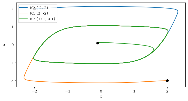
The Van der Pol oscillator is a prototypical nonlinear system that exhibits self-sustained oscillations. For a wide range of initial conditions, trajectories converge to a stable limit cycle.
In the form we will use in this course, the system is written as (Strogatz 2024, chap. 7.5):
\[\begin{aligned} \dot x &= \mu\,(y - f(x)) \\ \dot y &= -\frac{x}{\mu} \end{aligned} \tag{1}\]
where \(\mu>0\) controls the strength of the nonlinearity (and the fast–slow character for large \(\mu\)), and
\[ f(x) = \frac{x^3}{3} - x. \tag{2}\]
The nullclines are especially simple in this model:
\[ \dot x = 0 \quad \Longrightarrow \quad y = \frac{x^3}{3} - x, \qquad \dot y = 0 \quad \Longrightarrow \quad x = 0. \]
They intersect at the origin, so \((0,0)\) is the equilibrium point. For the parameter regime used in this session, the main long-run object of interest is not the equilibrium itself, but the attracting limit cycle around it.
scipy.integrate.solve_ivp() and matplotlib.
def van_der_pol(t, xy, mu=1.0):
    x, y = xy
    fx = x**3 / 3 - x
    dxdt = mu * (y - fx)
    dydt = -x / mu
    return np.array([dxdt, dydt])
Follow the same pipeline as in CDIMA Reaction: define the right-hand side, solve the initial value problem, compute nullclines, and then animate the resulting trajectory.
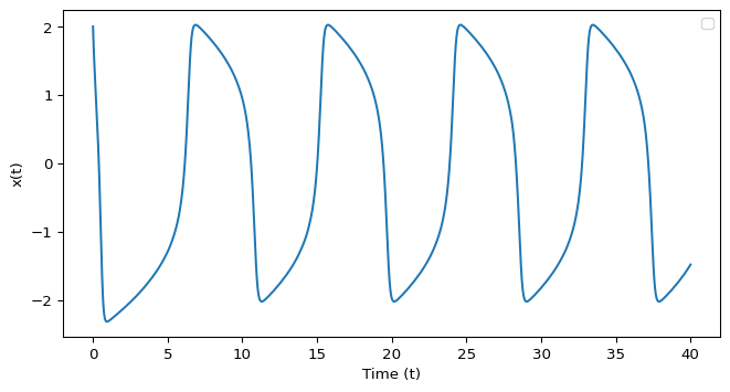
The Van der Pol system has a stable limit cycle that attracts trajectories from a wide range of initial conditions. Plot this limit cycle as a \(x(t)-t\) plot, and verify that it matches the phase plane trajectories.
/tmp/ipykernel_3383/2854713749.py:14: UserWarning:

No artists with labels found to put in legend.  Note that artists whose label start with an underscore are ignored when legend() is called with no argument.
scipy.integrate.solve_ivp() and matplotlib.
The amplitude and period of the limit cycle depend on \(\mu\).
This is the characteristic relaxation-oscillation picture.
Play with the parameter \(\mu\) to see how it changes the shape of the limit cycle and the transient dynamics.
Once the geometry is clear, the next step is to animate the trajectory and, if needed, make the initial condition interactive.