Spruce Budworm Model
1D Ordinary Differential Equations
The spruce budworm is an insect that periodically devastates spruce forests. The population dynamics can be modeled by the following ODE (Strogatz 2024, chap. 3.7):
\[ \frac{dx}{dt} = rx\left(1 - \frac{x}{k}\right) - \frac{x^2}{1 + x^2} \tag{1}\]
where:
- \(x(t)\) is the budworm population (adimensional).
- \(r\) is the intrinsic growth rate (typically \(r \approx 0.5\)).
- \(k\) is the carrying capacity of the forest (typically \(k \approx 10\)).
The first term represents logistic growth, while the second term models predation by birds (which follows a saturating functional response).
Implementing the ODE Function
Create a Python function that implements the spruce budworm differential equation. The function should follow the signature required by scipy.integrate.solve_ivp.
- Function name:
spruce_budworm - Parameters:
t(time),x(population),r(growth rate),k(carrying capacity) - Return: The rate of change \(\frac{dx}{dt}\).
- Include appropriate docstring documentation.
Here is a template to get you started:
def spruce_budworm(t: float, x: float, r: float = 0.5, k: float = 10) -> float:
    """Docstring and type hints"""
    # Your implementation here
    dxdt = # fill in the equation
    return dxdt
Why do we need t as an input? Although the equation does not explicitly depend on time, solve_ivp requires the function to accept time as the first argument.
Phase Portrait Visualization
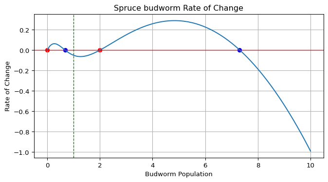
Create a function that plots the rate of change \(\frac{dx}{dt}\) as a function of the population \(x\). This phase portrait will help us visualize the equilibrium points and their stability.
- Function name:
plot_spruce_budworm_rate - Parameters:
x_t(current population),r,k - Use
matplotlibfor plotting - Plot \(\frac{dx}{dt}\) vs \(x\) for \(x \in [0, k]\)
- Identify and mark equilibrium points (where \(\frac{dx}{dt} = 0\))
- Color-code equilibrium points:
- Blue circles for stable equilibria (where \(\frac{dx}{dt}\) crosses zero from above).
- Red circles for unstable equilibria (where \(\frac{dx}{dt}\) crosses zero from below).
- Add a horizontal line at \(y = 0\) to indicate equilibria (null rate of change).
- Label axes and add a title.
- Mark the current population \(x_t\) with a vertical dashed line.
Figure 1 shows an example of the expected output.
Here are some hints to help you implement this function:
- You can use
np.linspaceto create an array of \(x\) values. - To find zero crossings: you can look for sign changes combining
np.diffandnp.sign. - Stability: a fixed point is stable if \(\frac{dx}{dt}\) decreases as you pass through it.
Review the following definitions for clarity:
- Equilibrium point: A value \(x^*\) where \(\frac{dx}{dt} = 0\).
- Stable equilibrium: Small perturbations decay back to \(x^*\).
- Unstable equilibrium: Small perturbations grow away from \(x^*\).
Numerical Integration
Create a function that evolves the system forward in time using numerical integration. This function should solve the ODE and append the results to existing time and population arrays.
- Function name:
evolve_spruce_budworm - Inputs:
t(time array),x(population array),r,k,t_eval(duration to evolve). - Use
scipy.integrate.solve_ivpwith the RK45 method. - Start from the last values in the input arrays.
- Concatenate new results to the input arrays.
- Ensure population never goes negative (use
np.clip). - Return updated
tandxarrays.
Here is a template to get you started:
def evolve_spruce_budworm(t: np.ndarray, x: np.ndarray, ...):
    """Don't forget the docstring and type hints"""
    # Define time span from last time point
    t_span = (t[-1], t[-1] + t_eval)

    # Create evaluation points, t_eval
    # This indicates where we want the solution evaluated
    # and should be distributed along the time span
    # Hint: use np.linspace

    # Solve the ODE
    solution = solve_ivp(
        fun=spruce_budworm,
        t_span=t_span,
        y0=[x[-1]],
        t_eval=t_eval,
        args=(r, k),
        method="RK45",
    )
    t_new = solution.t
    x_new = solution.y[0]

    # Concatenate results - Hint: use np.concatenate
    # Ensure non-negative population - Hint: use np.clip

    return t, x
Some important notes:
- The
argsparameter insolve_ivppasses additional arguments to your ODE function. You can see how we use it in the example above. - Initial condition should be
[x[-1]](last population value). - Use
method="RK45"for adaptive step-size Runge-Kutta integration.
Time Series Visualization
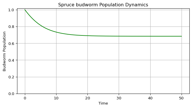
Create a function to plot the population dynamics over time. This visualization shows how the population evolves from the initial condition.
- Function name:
plot_spruce_budworm - Parameters:
t(time array),x(population array). - Plot time on the x-axis and population on the y-axis.
- Use green color for the trajectory.
- Ensure y-axis starts at 0 (populations cannot be negative).
- Include grid, labels, and title.
- Return the figure and axes objects.
See Figure 2 for an example output.
Building the Streamlit Application
Now that you have all the components, create an interactive Streamlit application that allows users to explore the spruce budworm model. This will enable real-time parameter adjustment and visualization.
While all the previous code could be done in Google Colab, Streamlit has to be built on your local machine. Follow the instructions in the README.md file in the repository to set up your environment.
Design a script, name it spruce_budworm_app.py. You will find a suggested layout below. This script will use the functions you implemented in sections Section 1 through Section 4. You can either import them from a separate module (another script you created) or paste the function definitions directly into the script. For best practices, consider creating a module (e.g., spruce_budworm_model.py) and importing the functions.
To test your app, run the following command in your terminal:
streamlit run spruce_budworm_app.pyInteractive Features
- Display the differential equation with current parameter values.
- Show the phase portrait (rate of change plot), using your function from section Section 2.
- Show the time series evolution, using your function from section Section 4.
- Add a button to “Evolve Forward” that continues the simulation, updating the plots.
- Use
st.session_stateto maintain simulation state between button clicks. You will need to store the time and population arrays in the session state, otherwise they will reset on each interaction.
Layout Structure
import streamlit as st
import numpy as np
import matplotlib.pyplot as plt
from your_module import (
    spruce_budworm,
    plot_spruce_budworm_rate,
    evolve_spruce_budworm,
    plot_spruce_budworm,
)  # Or paste your functions here

st.title("Spruce Budworm Population Dynamics")

# Sidebar parameters (as in the app)
r = st.sidebar.slider("Intrinsic growth rate (r)", 0.0, 1.0, 0.5)
k = st.sidebar.slider("Carrying capacity (k)", 0.1, 10.0, 10.0)

# The app sets the initial population to k/10 by default
x0 = k / 10

# Initialize session state
if ("sbw_x" not in st.session_state):
    st.session_state["sbw_t"] = np.array([0])
    st.session_state["sbw_x"] = np.array([x0])

# Time slider and control buttons
t_eval = st.sidebar.slider("Time", 1, 100, 10)
button = st.sidebar.button("Evolve")

# Retrieve session data
t = st.session_state["sbw_t"]
x = st.session_state["sbw_x"]

# Evolve if requested
if button:
    t, x = evolve_spruce_budworm(t, x, r=r, k=k, t_eval=t_eval)
    st.session_state["sbw_t"] = t
    st.session_state["sbw_x"] = x

# Plot phase portrait and time series
fig1, ax1 = plot_spruce_budworm_rate(x[-1], r=r, k=k)
st.pyplot(fig1)
fig2, ax2 = plot_spruce_budworm(t, x)
st.pyplot(fig2)
Advanced Features (Optional)
- Add a reset button to restart the simulation.
- Show multiple trajectories with different initial conditions.
- Add animation of the population dynamics.
Exploration Questions
Once your simulation is working, explore the following questions:
- Multiple Equilibria: For \(r = 0.5\) and \(k = 10\), how many equilibrium points exist? Which are stable?
- Bistability: Start with two different initial conditions (e.g., \(x_0 = 1\) and \(x_0 = 8\)). Do they converge to the same equilibrium?
- Hysteresis: Slowly increase the carrying capacity \(k\) from 5 to 15. Then slowly decrease it back to 5. Does the population return to the same state? If you are interested in this concept, see section Section 6.1.
- Outbreak Dynamics: What happens if you start with a small population (\(x_0 < 2\)) and the carrying capacity is large (\(k > 10\))?
- Critical Slowing Down: When the population is near an unstable equilibrium, how long does it take to move away? Compare this to the rate of change far from equilibrium.
- Parameter Space: Create a diagram showing the number of equilibria as a function of \(r\) and \(k\). Where do bifurcations occur?
Slow-Fast Dynamics
The carrying capacity \(k\) can be interpreted as a slowly varying parameter in real ecosystems (e.g., due to seasonal changes or forest management). You can simulate this by gradually changing \(k\) over time in your app. This can lead to hysteresis effects, where the population does not return to its original state after \(k\) is restored. Experiment with this by modifying your Streamlit app to allow \(k\) to vary over time.
Mathematical Background
In this section I provide some additional mathematical context for the spruce budworm model. Play with your simulation to see these concepts in action!
Equilibrium Analysis
Equilibrium points satisfy:
\[ rx^*\left(1 - \frac{x^*}{k}\right) - \frac{(x^*)^2}{1 + (x^*)^2} = 0 \tag{2}\]
This can be rewritten as:
\[ rx^*\left(1 - \frac{x^*}{k}\right) = \frac{(x^*)^2}{1 + (x^*)^2} \tag{3}\]
The left side represents birth rate (logistic growth), and the right side represents predation rate. Equilibria occur where these balance.
Stability Analysis
The stability of an equilibrium \(x^*\) is determined by the sign of the derivative:
\[ \frac{d}{dx}\left(\frac{dx}{dt}\right)\bigg|_{x=x^*} \tag{4}\]
If this derivative is:
- Negative: the equilibrium is stable (attracting).
- Positive: the equilibrium is unstable (repelling).
- Zero: higher-order analysis is needed.
Ecological Interpretation
- Low equilibrium: Few budworms, controlled by predation.
- High equilibrium: Outbreak state, budworms overwhelm predators.
- Middle equilibrium: Usually unstable, separates the two basins of attraction.
- Hysteresis: The system can “jump” between states depending on history.
This behavior explains why spruce budworm populations can suddenly explode from low levels to outbreak proportions, and why simply reducing the outbreak may not return the forest to a healthy state.
Resources
- (Strogatz 2024, chap. 3.7) for theoretical background on the spruce budworm model.
- SciPy documentation: https://docs.scipy.org/doc/scipy/reference/generated/scipy.integrate.solve_ivp.html
- Streamlit documentation: https://docs.streamlit.io
- Reference implementation: https://github.com/daniprec/BAM-Applied-Math-Lab/tree/main/amlab/odes_1d
References
Strogatz, Steven H. 2024. Nonlinear Dynamics and Chaos: With Applications to Physics, Biology, Chemistry, and Engineering. Chapman; Hall/CRC.