Gierer-Meinhardt Model (2D)
Reaction-Diffusion PDE
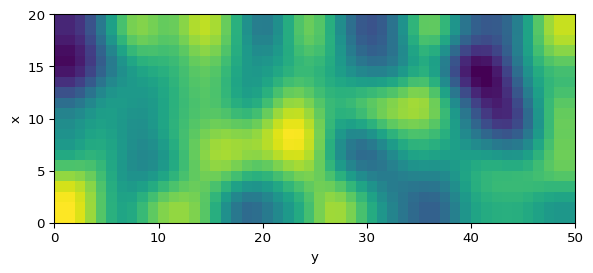
The 2D Gierer-Meinhardt model is a pattern-forming reaction-diffusion system. We will extend the 1D solver to a rectangular domain \(\Omega = (0, L_1) \times (0, L_2)\) and visualize \(v(x,y)\).
In 2D the model is
\[ \begin{aligned} \frac{\partial u}{\partial t} &= \Delta u + \gamma \left(a - b u + \frac{u^2}{v}\right), \\ \frac{\partial v}{\partial t} &= d\,\Delta v + \gamma \left(u^2 - v\right), \end{aligned} \tag{1}\]
where \(u(x,y,t)\) and \(v(x,y,t)\) are concentrations.
Laplacian in 2D
In two dimensions the Laplacian is
\[ \Delta u = \frac{\partial^2 u}{\partial x^2} + \frac{\partial^2 u}{\partial y^2}. \tag{2}\]
Using a 5-point stencil with spacing \(h\):
\[ \Delta u(x,y) \approx \frac{u(x+h,y) + u(x-h,y) + u(x,y+h) + u(x,y-h) - 4u(x,y)}{h^2}. \tag{3}\]
A 9-point stencil improves accuracy by including diagonal neighbors:
\[ \Delta u(x,y) \approx \frac{-20u(x,y) + 4\sum_{\text{cardinal}} u + \sum_{\text{diagonal}} u}{6h^2}. \tag{4}\]
Exercise: Simulate the PDE
We will use \(L_1=20\), \(L_2=50\), \(dx=1\), \(dt=0.001\), \(a=0.40\), \(b=1.00\), \(d=20\), and \(\gamma=1\). Follow the steps below and compare your output to Figure 1.
Initialize the fields
import numpy as np

length_x = 20
length_y = 50
dx = 1
lenx = int(length_x / dx)
leny = int(length_y / dx)

uv = np.ones((2, lenx, leny))
uv += uv * np.random.uniform(0, 1, uv.shape) / 100
Define the PDE (template)
def gierer_meinhardt_pde(t, uv, gamma=1, a=0.40, b=1.00, d=20, dx=1):
    # TODO: compute the 2D Laplacian with np.roll

    # TODO: implement the reaction terms f(u, v) and g(u, v)
    # TODO: combine diffusion + reaction to build du_dt and dv_dt
    return du_dt, dv_dt
Hint: Gierer-Meinhardt 2D PDE (click to expand)
def gierer_meinhardt_pde(t, uv, gamma=1, a=0.40, b=1.00, d=20, dx=1):
    lap = -4 * uv
    lap += np.roll(uv, shift=1, axis=1)
    lap += np.roll(uv, shift=-1, axis=1)
    lap += np.roll(uv, shift=1, axis=2)
    lap += np.roll(uv, shift=-1, axis=2)
    lap /= dx**2

    u, v = uv
    lu, lv = lap

    f = a - b * u + (u**2) / v
    g = u**2 - v
    du_dt = lu + gamma * f
    dv_dt = d * lv + gamma * g
    return du_dt, dv_dt
Time stepping (template)
num_iter = 50000
dt = 0.001

for _ in range(num_iter):
    dudt, dvdt = gierer_meinhardt_pde(0, uv, dx=dx)
    # TODO: update u and v with Euler's method

    # TODO: enforce Neumann boundary conditions in both directions
Plot the image (template)
import matplotlib.pyplot as plt

fig, ax = plt.subplots()
im = ax.imshow(
    uv[1],
    interpolation="bilinear",
    origin="lower",
    extent=[0, length_y, 0, length_x],
)
plt.show()
Animation
Instead of running a long loop, move the Euler updates inside the animation callback.
import matplotlib.animation as animation
import matplotlib.pyplot as plt

fig, ax = plt.subplots()
im = ax.imshow(uv[1], origin="lower", extent=[0, length_y, 0, length_x])

def update_animation(frame):
    # TODO: update uv via Euler steps
    # TODO: apply Neumann boundary conditions
    im.set_array(uv[1])
    im.set_clim(vmin=uv[1].min(), vmax=uv[1].max() + 0.1)
    return (im,)

ani = animation.FuncAnimation(fig, update_animation, interval=1, blit=True)
Hint: Animation update (click to expand)
def update_animation(frame):
    global uv
    for _ in range(anim_speed):
        dudt = gierer_meinhardt_pde(0, uv, gamma=gamma, a=a, b=b, d=d, dx=dx)
        uv = uv + dudt * dt
        uv[:, 0, :] = uv[:, 1, :]
        uv[:, -1, :] = uv[:, -2, :]
        uv[:, :, 0] = uv[:, :, 1]
        uv[:, :, -1] = uv[:, :, -2]

    im.set_array(uv[1])
    im.set_clim(vmin=uv[1].min(), vmax=uv[1].max() + 0.1)
    return (im,)
Explore
Try different parameter values for \((a, d)\) and describe the pattern. What changes when you increase \(d\)?