Gierer-Meinhardt Model (1D)
Reaction-Diffusion PDE
The Gierer-Meinhardt model is a classical reaction-diffusion system that can generate spatial patterns. We will build a 1D solver from scratch and visualize \(v(x)\).
In 1D it reads
\[ \begin{aligned} \frac{\partial u}{\partial t} &= \Delta u + \gamma \left(a - b u + \frac{u^2}{v}\right), \\ \frac{\partial v}{\partial t} &= d\,\Delta v + \gamma \left(u^2 - v\right), \end{aligned} \tag{1}\]
where \(u(x,t)\) and \(v(x,t)\) are concentrations, \(a,b,\gamma\) are reaction parameters, and \(d\) is the diffusion ratio for \(v\).
Laplacian in 1D
In one dimension, the Laplacian is the second derivative:
\[ \Delta u = \frac{d^2 u}{dx^2}. \tag{2}\]
Using a centered finite difference on a grid with spacing \(h\):
\[ \Delta u(x) \approx \frac{u(x+h) - 2u(x) + u(x-h)}{h^2} + \mathcal{O}(h^2). \tag{3}\]
This is easy to implement with np.roll() to access neighbors on a grid. We will assume \(h = dx\) and use the second-order centered difference.
Boundary Conditions
Neumann (zero flux)
\[u_x(0)=0,\quad u(0)=u(h) \tag{4}\]
Dirichlet (fixed values)
\[u(0)=\alpha,\quad u(L)=\beta \tag{5}\]
Periodic
\[u(0)=u(L) \tag{6}\]
Exercise: Simulate the PDE
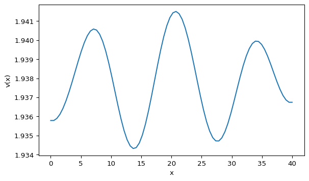
We will use \(L=40\), \(dx=0.5\), \(dt=0.001\), \(a=0.40\), \(b=1.00\), \(d=20\), and \(\gamma=1\). Follow the steps below and compare your result with Figure 1.
Initialize the fields
import numpy as np

length = 40
dx = 0.5
lenx = int(length / dx)

uv = np.ones((2, lenx))
uv += uv * np.random.randn(2, lenx) / 100
Why add noise? A perfectly uniform initial condition can hide instabilities. Small perturbations reveal pattern-forming behavior.
Define the PDE (template)
def gierer_meinhardt_pde(t, uv, gamma=1, a=0.40, b=1.00, d=20, dx=1):
    # Laplacian via finite differences (np.roll handles neighbors)
    lap = -2 * uv
    lap += np.roll(uv, shift=1, axis=1)
    lap += np.roll(uv, shift=-1, axis=1)
    lap /= dx**2

    u, v = uv
    lu, lv = lap

    # TODO: implement the reaction terms f(u, v) and g(u, v)
    # TODO: combine diffusion + reaction to build du_dt and dv_dt
    return du_dt, dv_dt
Hint: Gierer-Meinhardt PDE (click to expand)
def gierer_meinhardt_pde(t, uv, gamma=1, a=0.40, b=1.00, d=20, dx=1):
    lap = -2 * uv
    lap += np.roll(uv, shift=1, axis=1)
    lap += np.roll(uv, shift=-1, axis=1)
    lap /= dx**2

    u, v = uv
    lu, lv = lap

    f = a - b * u + (u**2) / v
    g = u**2 - v
    du_dt = lu + gamma * f
    dv_dt = d * lv + gamma * g
    return du_dt, dv_dt
Time stepping (template)
num_iter = 50000
dt = 0.001

for _ in range(num_iter):
    dudt, dvdt = gierer_meinhardt_pde(0, uv, dx=dx)
    # TODO: update u and v with Euler's method

    # TODO: enforce Neumann boundary conditions
Plot the final profile (template)
import matplotlib.pyplot as plt

x = np.linspace(0, length, lenx)
fig, ax = plt.subplots()
ax.plot(x, uv[1])
ax.set_xlabel("x")
ax.set_ylabel("v(x)")
ax.set_title("Gierer-Meinhardt 1D")
plt.show()
Explore
Re-run with \(d=30\) and compare the pattern. Try other \((a, d)\) pairs and share your observations.
Animation Extension
Instead of plotting only the final state, update the line at every frame:
import matplotlib.animation as animation

(plot_v,) = ax.plot(x, uv[1])

def animate(frame):
    nonlocal uv
    # TODO: compute dudt, dvdt and update uv
    # TODO: update the line data
    return (plot_v,)

ani = animation.FuncAnimation(fig, animate, interval=1, blit=True)
Hint: Animation update (click to expand)
def animate(frame):
    nonlocal uv
    dudt, dvdt = gierer_meinhardt_pde(frame, uv, dx=dx)
    uv[0] = uv[0] + dudt * dt
    uv[1] = uv[1] + dvdt * dt
    plot_v.set_data(x, uv[1])
    return (plot_v,)
If the system stays flat for some parameters and forms waves for others, you are seeing the onset of Turing instability. Proceed to the next page to analyze it.
Tip
Full reference code is available in amlab/pdes_1d.