Gray-Scott Model
Build Your Own 2D Reaction-Diffusion Simulator
The Gray-Scott model is one of the cleanest examples of reaction-diffusion pattern formation. It combines diffusion with an autocatalytic reaction and produces spots, stripes, worms, and labyrinths depending on the parameters (Gray and Scott 1984; Pearson 1993).
This is the next step after the 2D Gierer-Meinhardt page. The grid, the Laplacian, and the Euler loop are the same. The new ingredient is the reaction term, which is simple to write and much richer visually.
Conceptually, the jump from Gierer-Meinhardt to Gray-Scott is small.
- The domain is still a rectangular 2D grid.
- The Laplacian is still the same vectorized 5-point stencil.
- Time stepping is still explicit Euler.
- The main numerical change is the boundary condition: here we keep the periodic wrapping built into
np.roll()instead of overwriting the edges with Neumann data.
That is why this page should feel familiar. Once the Gierer-Meinhardt solver works, you mostly change the reaction terms and the interpretation of the boundary.
The PDE system is
\[ \begin{aligned} \frac{\partial u}{\partial t} &= d_1 \Delta u - u v^2 + f(1-u), \\ \frac{\partial v}{\partial t} &= d_2 \Delta v + u v^2 - (f+k) v, \end{aligned} \tag{1}\]
where \(d_1\) and \(d_2\) are the diffusion coefficients, \(f\) is the feed rate, and \(k\) is the kill rate.
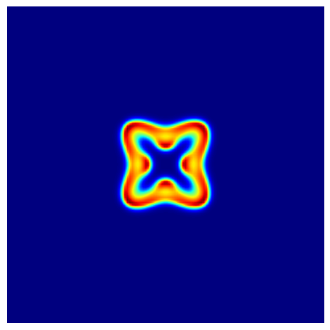
Start from the Homogeneous State
Gray-Scott is usually initialized near the steady state \((u, v) = (1, 0)\), then a small patch is perturbed.
import numpy as np

n = 250
dt = 2.0
uv = np.ones((2, n, n), dtype=np.float32)
uv[1] = 0.0

c = n // 2
r = 12

# TODO: perturb a square patch around the center
# Set u close to 0.5 and v close to 0.25 in that patch

# TODO: add 10% Gaussian noise inside the same patch
Hint: Gray-Scott initialization (click to expand)
uv[0, c - r : c + r, c - r : c + r] = 0.5
uv[1, c - r : c + r, c - r : c + r] = 0.25

noise = 0.1 * np.random.randn(2, 2 * r, 2 * r)
uv[:, c - r : c + r, c - r : c + r] *= 1 + noise
Reuse the 2D Laplacian
We will start with the 5-point stencil. If you implemented the previous page cleanly, you can reuse that helper almost unchanged.
import numpy as np

def laplacian(field):
    # TODO: write the 5-point stencil with np.roll
    return lap
Hint: 5-point stencil (click to expand)
def laplacian(field):
    lap = -4 * field
    lap += np.roll(field, shift=1, axis=0)
    lap += np.roll(field, shift=-1, axis=0)
    lap += np.roll(field, shift=1, axis=1)
    lap += np.roll(field, shift=-1, axis=1)
    return lap
The only reason this already enforces periodic boundary conditions is that np.roll() wraps the array. If you wanted zero-flux or fixed-value boundaries here, you would keep the same Laplacian helper and reuse the boundary-update pattern from the 2D Gierer-Meinhardt page after every Euler step.
Implement the Gray-Scott PDE
import numpy as np

def gray_scott_pde(t, uv, d1=0.1, d2=0.05, f=0.040, k=0.060):
    u, v = uv
    lu = laplacian(u)
    lv = laplacian(v)

    # TODO: compute the autocatalytic term uv^2
    uv2 =

    # TODO: write du_dt and dv_dt
    du_dt =
    dv_dt =
    return np.array([du_dt, dv_dt])
Hint: Gray-Scott PDE (click to expand)
def gray_scott_pde(t, uv, d1=0.1, d2=0.05, f=0.040, k=0.060):
    u, v = uv
    lu = laplacian(u)
    lv = laplacian(v)
    uv2 = u * v * v

    du_dt = d1 * lu - uv2 + f * (1 - u)
    dv_dt = d2 * lv + uv2 - (f + k) * v
    return np.array([du_dt, dv_dt])
Time Step and Animate
Because np.roll() wraps around the array, this implementation already uses periodic boundary conditions.
This is the main conceptual difference from the previous page. There, we copied the edge values after each Euler step to model zero flux. Here, we let the pattern leave one side of the domain and re-enter on the opposite side.
import matplotlib.animation as animation
import matplotlib.pyplot as plt

fig, ax = plt.subplots(figsize=(6, 6))
im = ax.imshow(uv[1], cmap="jet", interpolation="bilinear", vmin=0, vmax=1)
ax.axis("off")

def update_frame(_):
    # TODO: advance uv by one or more Euler steps
    im.set_array(uv[1])
    return [im]

ani = animation.FuncAnimation(fig, update_frame, interval=1, blit=True)
Hint: Gray-Scott animation (click to expand)
def update_frame(_):
    nonlocal uv
    for _ in range(20):
        uv = uv + gray_scott_pde(0, uv, d1=0.1, d2=0.05, f=0.040, k=0.060) * dt
    im.set_array(uv[1])
    return [im]
Parameter Sets
Try the following values with \(d_1 = 0.1\) and \(d_2 = 0.05\):
- Type A: \(f = 0.040\), \(k = 0.060\)
- Type B: \(f = 0.014\), \(k = 0.047\)
- Type C: \(f = 0.062\), \(k = 0.065\)
- Type D: \(f = 0.078\), \(k = 0.061\)
- Type E: \(f = 0.082\), \(k = 0.059\)
Which sets create isolated spots? Which ones create stripes or moving fronts?
Connection Back to Turing Analysis
The same steady-state to Jacobian to mode-matrix pipeline from the Turing page still applies here. The only spectral change is the boundary condition.
- For Neumann boundaries, the admissible wavenumbers use factors of \(\pi / L\).
- For periodic boundaries, the admissible wavenumbers use factors of \(2\pi / L\).
For the usual base state \((u, v) = (1, 0)\), the linearized system is damped, so the classical Turing calculation only becomes interesting at a nontrivial homogeneous equilibrium when one exists. In that regime, the mode matrices are built exactly as before, but with the periodic Laplacian eigenvalues. That is the clean conceptual bridge from Gierer-Meinhardt to Gray-Scott.
Optional: 9-Point Stencil
If you want to compare stencils, adapt your Laplacian to include diagonal neighbors and compare the visual effect.
What’s Next?
The base solver is done. In the next page, we will keep the same PDE update and wrap it with interaction: drawing perturbations, pausing the simulation, and changing parameters with sliders.
Tip
Reference code is available in amlab/pdes/gray_scott.py.
References
Gray, Peter, and Stephen K. Scott. 1984. “Autocatalytic Reactions in the Isothermal, Continuous Stirred Tank Reactor: Isolas and Other Forms of Multistability.” Chemical Engineering Science 39 (6): 1087–97. https://doi.org/10.1016/0009-2509(84)87017-7.
Pearson, John E. 1993. “Complex Patterns in a Simple System.” Science 261 (5118): 189–92. https://doi.org/10.1126/science.261.5118.189.