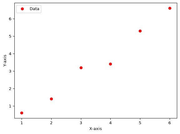
You have a set of points in a 2D plane, defined by the array pts.
The code below defines the points and plots them.
import matplotlib.pyplot as pltimport numpy as nppts = np.array([[1, 2, 3, 4, 5, 6], [0.6, 1.4, 3.2, 3.4, 5.3, 6.6]])# The following code uses matplotlib# You will learn about it in the 2nd semesterplt.plot(pts[0], pts[1], 'ro', label="Data")plt.legend()plt.xlabel("X-axis")plt.ylabel("Y-axis")plt.show()plt.close()
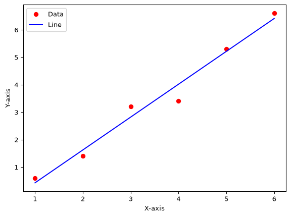
Assuming a set of \(N\) points \((xi, yi)\), we can try to fit a straight line so that:
# Solution# Extract x and y from the set of pointsx, y = pts# Generate the matrix Xones = np.ones(len(x))X = np.vstack([ones, x]).T# Compute the matrix# @ = np.matmulb = np.linalg.inv(X.T @ X) @ X.T @ y# Now we can use the vector b to estimate any value of y# Lets visuallize the line defined by bx_line = np.linspace(x[0], x[-1], 100)y_line = b[0] + b[1] * x_line# The following code uses matplotlib# You will learn about it in the 2nd semesterplt.plot(x, y, 'ro', label="Data")plt.plot(x_line, y_line, 'b-', label="Line")plt.legend()plt.xlabel("X-axis")plt.ylabel("Y-axis")plt.show()
Source Code
---title: "Review: Linear Regression"subtitle: "Module 4: IDEs & Tools"format: html---## Linear RegressionYou have a set of points in a 2D plane, defined by the array `pts`.The code below defines the points and plots them.```{python}import matplotlib.pyplot as pltimport numpy as nppts = np.array([[1, 2, 3, 4, 5, 6], [0.6, 1.4, 3.2, 3.4, 5.3, 6.6]])# The following code uses matplotlib# You will learn about it in the 2nd semesterplt.plot(pts[0], pts[1], 'ro', label="Data")plt.legend()plt.xlabel("X-axis")plt.ylabel("Y-axis")plt.show()plt.close()```Assuming a set of $N$ points $(xi, yi)$, we can try to fit a straight line so that:$$y_i = b_0 + b_1 \cdot x_i,\qquad \forall i \in [1, N]$$In matrix notation, the equation above is:$$\mathbf{Y} = X \cdot \mathbf{b}$$where:$$\mathbf{Y} = (y_1, ..., y_N)$$$$X = \begin{pmatrix}1 & x_1 \\...\\1 & x_N\end{pmatrix}$$$$\mathbf{b} = (b_0, b_1)$$We will use the Ordinary Least Squares method to fit the points in `pts`. Compute $\mathbf{b}$ using the Normal Equation:$$b = \left(X^T \cdot X\right)^{-1} \cdot X^T \cdot Y$$```{python}# Solution# Extract x and y from the set of pointsx, y = pts# Generate the matrix Xones = np.ones(len(x))X = np.vstack([ones, x]).T# Compute the matrix# @ = np.matmulb = np.linalg.inv(X.T @ X) @ X.T @ y# Now we can use the vector b to estimate any value of y# Lets visuallize the line defined by bx_line = np.linspace(x[0], x[-1], 100)y_line = b[0] + b[1] * x_line# The following code uses matplotlib# You will learn about it in the 2nd semesterplt.plot(x, y, 'ro', label="Data")plt.plot(x_line, y_line, 'b-', label="Line")plt.legend()plt.xlabel("X-axis")plt.ylabel("Y-axis")plt.show()```---