Initial value problems, nonlinear rate laws, and a reusable solver workflow
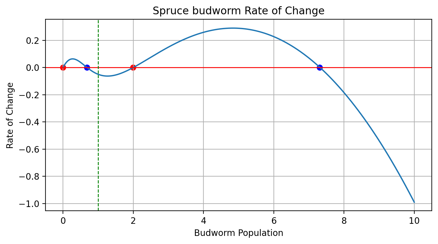
The first session sets the numerical pattern for the whole lab: define a model, choose initial data, integrate forward, and interpret what the trajectory means.
IVP
\[ \dot y = f(t, y), \qquad y(t_0) = y_0 \]
Use the same solve_ivp() pipeline in epidemic models, chemical kinetics, and population dynamics.
You leave this session with a template that you will reuse in later ODE, synchronization, and PDE topics.
Write the right-hand side, define t_span, choose y0, and inspect the output carefully.
See how even a small coupled system still fits the same initial value problem pipeline.
Study saturation and threshold effects in Michaelis-Menten style kinetics and the spruce budworm model.
Write a function fun(t, y) that returns the rate law.
Choose parameters, a time interval, and an initial state.
Integrate with solve_ivp() and sample the solution on a useful time grid.
Plot the trajectory and ask which parameters or initial conditions changed the outcome.
\[ \dot y = f(t, y), \qquad y(t_0) = y_0 \]
scipy.integrate.solve_ivp
The main numerical integrator for initial value problems in the course.
numpy
For initial conditions, parameter arrays, time grids, and vectorized post-processing.
matplotlib.pyplot
For time series, parameter comparisons, and phase-line style interpretation.
\[ \dot S = -\beta S I, \quad \dot I = \beta S I - \gamma I, \quad \dot R = \gamma I \]
Track growth, peak prevalence, and the role of \(R_0 = \beta / \gamma\).
\[ v(S) = \frac{V_{\max} S}{K_m + S} \]
Use this to discuss why many rates stop growing linearly at large substrate levels.
\[ \dot x = r x \left(1 - \frac{x}{k}\right) - \frac{x^2}{1 + x^2} \]
This is the cleanest example of threshold behavior and bistability in the session.
Use the full module page when you want the phase-line analysis and parameter exploration.

import numpy as np
from scipy.integrate import solve_ivp
def rhs(t, y, rate):
return -rate * y
t_eval = np.linspace(0.0, 10.0, 200)
sol = solve_ivp(rhs, (0.0, 10.0), y0=[2.0], t_eval=t_eval, args=(0.5,))Keep this pattern in mind. Most later solver-based sessions are variations on this same structure.
Use the deck for the lecture flow, then move to the module pages for derivations, code walkthroughs, and exercises.
Applied Math Lab