Creating Your Own Library
Module 4: IDEs & Tools
From a script to a library
In this section we will build a small library, step by step, and install it in our environment, just like NumPy or matplotlib.
Our running example is linear regression. You met it in the General Review: given \(N\) points \((x_i, y_i)\), we look for the line
\[y_i = b_0 + b_1 \cdot x_i\]
that fits them as well as possible. In matrix notation \(\mathbf{Y} = X \cdot \mathbf{b}\), where
\[ X = \begin{pmatrix} 1 & x_1 \\ \vdots & \vdots \\ 1 & x_N \end{pmatrix}, \qquad \mathbf{b} = \begin{pmatrix} b_0 \\ b_1 \end{pmatrix} \]
With the Ordinary Least Squares method we get \(\mathbf{b}\) from the Normal Equation:
\[\mathbf{b} = \left(X^T \cdot X\right)^{-1} \cdot X^T \cdot \mathbf{Y}\]
Step 1: the project folder and the first module
- Make sure your environment (for example
demo_env) has NumPy installed. - Create a folder called
my_first_libraryand open its parent folder in VS Code. - Inside it, create a script
regression.py.
import numpy as np


def linear_regression(x, y):
    """Fit y = b0 + b1 * x with the Normal Equation and return b."""
    x = np.asarray(x, dtype=float)
    y = np.asarray(y, dtype=float)
    X = np.column_stack([np.ones(len(x)), x])
    return np.linalg.inv(X.T @ X) @ X.T @ y


def main(points_file, output_file):
    """Read the points from a text file and save the coefficients b."""
    x, y = np.loadtxt(points_file, unpack=True)
    b = linear_regression(x, y)
    np.savetxt(output_file, b)
    print(f"b0 = {b[0]:.4f}, b1 = {b[1]:.4f}")


if __name__ == "__main__":
    main("data_array.txt", "b.txt")
The input file data_array.txt has one point per row, with x and y separated by a space:
1.0 2.1
2.0 3.9
3.0 6.2
4.0 7.8Python looks for data_array.txt in the working directory, which is normally the folder open in VS Code. Put the data file in that folder, or give a path to it (see Files and Directories).
Create data_array.txt with your own points, run regression.py, and check the file b.txt. Compare your result with the line that you get from the review exercise.
For example, create data_array.txt in the same folder as regression.py, with one point per row (x and y separated by a space):
1.0 2.1
2.0 3.9
3.0 6.2
4.0 7.8
Run the script:
python regression.py
# b0 = 0.1500, b1 = 1.9400
The file b.txt appears in the same folder with the two coefficients, one per row. They define the line \(y = 0.15 + 1.94\,x\), which is the line that passes closest to the four points.
To check it, fit the same points with NumPy:
import numpy as np

x, y = np.loadtxt("data_array.txt", unpack=True)
print(np.polyfit(x, y, 1))   # [1.94 0.15]  (slope first, then intercept)
np.polyfit returns the coefficients in the opposite order, but the numbers are the same.
Step 2: make it a package
We want to import our code from anywhere, not only from the folder where the file is. First we turn the folder into a package.
Create an empty file named __init__.py inside my_first_library. This file tells Python that the folder is a package. It can be empty, or contain code that runs when the package is imported.
Each script inside the package is now a module. We can import our function with:
from my_first_library.regression import linear_regressionYou could already import scripts before. The difference is that, once the library is installed (step 4), it does not matter where the script is located.
Your folder should look like this:
my_first_library/          <- project folder
├── my_first_library/      <- the package
│   ├── __init__.py
│   └── regression.py
├── setup.py
└── requirements.txt
Note that there are two folders with the same name: the outer one is the project, and the inner one is the package.
Step 3: setup file and requirements
Outside the package folder (in the project folder), create setup.py. It tells setuptools how to build and install your library, and includes metadata such as the name, version or author:
from setuptools import find_packages, setup

setup(
    name="my_first_library",
    version="0.1",
    packages=find_packages(),
    # More metadata: author, description, ...
)
If your library needs other packages, list them in requirements.txt, one per line. You can ask for the latest version or a specific one:
numpy
typer
To make pip install these dependencies automatically, add them to setup.py too:
setup(
    name="my_first_library",
    version="0.1",
    packages=find_packages(),
    install_requires=["numpy", "typer"],
)setup.py and pyproject.toml
setup.py is the classic way to describe a package and it is simple to understand, so we use it here. New projects often put the same information in a file called pyproject.toml, which is the current standard. The ideas (name, version, packages, dependencies) are the same.
Step 4: install your library
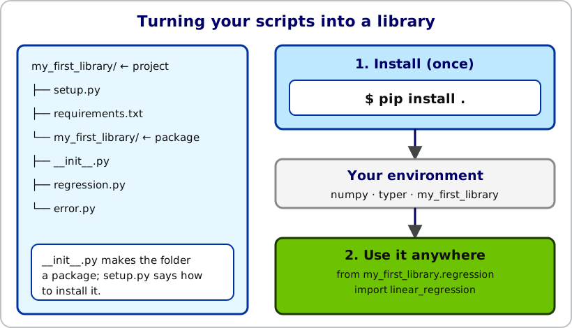
Open a terminal in the project folder (the one that contains setup.py), activate your environment and run:
pip install .The dot means “the current folder”. Now your library is installed in the environment. From any folder, script or notebook using that environment you can write:
from my_first_library.regression import linear_regression

print(linear_regression([1, 2, 3, 4], [3, 5, 7, 9])) # [1. 2.]If you change the code of your library, install it again with pip install .. A more comfortable option while developing is pip install -e . (editable mode), which makes Python use your files directly, so changes apply immediately.
Step 5: command-line options with typer
Our main has the file names written in the code. How can the user choose a different file when running the script? The typer library (install it with pip) turns the arguments of a function into command-line options.
import typer


def main(name: str = "Daniel"):
    print(f"Name is {name}")


if __name__ == "__main__":
    typer.run(main)
Save this as demo.py and run it:
python demo.py
# Name is Daniel

python demo.py --name Bella
# Name is Bella
Every parameter of main becomes an option (--name), and its type hint (str) tells typer how to convert it. Parameters with a default value are optional.
Let’s use it in regression.py. Replace the last lines with:
import typer


def main(points_file: str = "data_array.txt", output_file: str = "b.txt"):
    """Read the points from a text file and save the coefficients b."""
    x, y = np.loadtxt(points_file, unpack=True)
    b = linear_regression(x, y)
    np.savetxt(output_file, b)
    print(f"b0 = {b[0]:.4f}, b1 = {b[1]:.4f}")


if __name__ == "__main__":
    typer.run(main)
Now we can choose the files from the terminal (--points-file uses a hyphen):
python regression.py --points-file my_points.txt --output-file my_b.txtStep 6: add a new module
A library usually has several modules. Create error.py inside the package. It will measure how good the fit is, using two standard measures for points \(y_i\) and predictions \(\hat{y}_i\):
\[ L_1 = \frac{1}{N}\sum_i \left|y_i - \hat{y}_i\right|, \qquad L_2 = \sqrt{\frac{1}{N}\sum_i \left(y_i - \hat{y}_i\right)^2} \]
Write my_first_library/error.py with:
- the functions
l1_error(y_true, y_pred)andl2_error(y_true, y_pred), which take NumPy arrays and return floats; - a
mainfunction that takes two files, the array of points \((x, y)\) and the file with the coefficients \(\mathbf{b}\), and prints the L1 and L2 errors.
import numpy as np
import typer


def l1_error(y_true, y_pred):
    """Mean absolute error."""
    return float(np.mean(np.abs(np.asarray(y_true) - np.asarray(y_pred))))


def l2_error(y_true, y_pred):
    """Root mean squared error."""
    return float(np.sqrt(np.mean((np.asarray(y_true) - np.asarray(y_pred)) ** 2)))


def main(points_file: str, coefficients_file: str):
    x, y = np.loadtxt(points_file, unpack=True)
    b = np.loadtxt(coefficients_file)
    y_pred = b[0] + b[1] * x
    print(f"L1 error: {l1_error(y, y_pred):.4f}")
    print(f"L2 error: {l2_error(y, y_pred):.4f}")


if __name__ == "__main__":
    typer.run(main)
Run it with python error.py data_array.txt b.txt. Remember to reinstall the library (pip install .) after adding a module.
Step 7: use your library in a notebook
- Open a new notebook and select your environment (
demo_env) as the kernel. - Import NumPy,
linear_regression,l1_errorandl2_error. - Load
data_array.txtinto arraysxandy, fit the model and compute the L1 and L2 errors.
import numpy as np

from my_first_library.regression import linear_regression
from my_first_library.error import l1_error, l2_error

x, y = np.loadtxt("data_array.txt", unpack=True)
b = linear_regression(x, y)
y_pred = b[0] + b[1] * x

print(b)
print(l1_error(y, y_pred), l2_error(y, y_pred))
Challenges
Extend linear_regression so that it accepts a matrix of inputs with any number of columns:
\[y_i = b_0 + b_1 x_{1,i} + b_2 x_{2,i} + \dots\]
Hint: build \(X\) with a first column of ones followed by one column per variable, and use the same Normal Equation.
import numpy as np


def linear_regression(X_inputs, y):
    """Fit y = b0 + b1 * x1 + b2 * x2 + ... and return b.

    X_inputs has shape (N,) for one variable, or (N, k) for k variables.
    """
    X_inputs = np.asarray(X_inputs, dtype=float)
    if X_inputs.ndim == 1:
        X_inputs = X_inputs[:, None]
    X = np.column_stack([np.ones(len(X_inputs)), X_inputs])
    return np.linalg.solve(X.T @ X, X.T @ np.asarray(y, dtype=float))
The first column of ones gives the intercept \(b_0\), and each extra column of X_inputs adds one coefficient. Using np.linalg.solve instead of an explicit inverse is faster and numerically more stable, and gives the same result. The function still works with one variable, so your earlier code does not break.
In the same notebook, use NumPy to generate:
x1: 100 random points in the interval \([0, 10]\).x2: 100 random points in the interval \([20, 40]\).- \(y = 3 + 4 x_1 - x_2\).
- Noisy values \(y' = y + N(0, 2)\) (a normal distribution with mean 0 and standard deviation 2).
Fit \((x_1, x_2, y')\) with your regression and compute the L1 and L2 errors. What happens to the errors when you use 1,000,000 points instead of 100?
Hint: use the function from Challenge 1.
import numpy as np

from my_first_library.error import l1_error, l2_error

# linear_regression is the extended version from Challenge 1
from my_first_library.regression import linear_regression

rng = np.random.default_rng(0)
n = 100          # try also 1_000_000
x1 = rng.uniform(0, 10, n)
x2 = rng.uniform(20, 40, n)
y = 3 + 4 * x1 - x2
y_noisy = y + rng.normal(0, 2, n)

b = linear_regression(np.column_stack([x1, x2]), y_noisy)
y_pred = b[0] + b[1] * x1 + b[2] * x2

print(b)                          # close to [3, 4, -1]
print(l1_error(y_noisy, y_pred))  # about 1.7 (n = 100)
print(l2_error(y_noisy, y_pred))  # about 2.2 (n = 100)
(To use the extended function from the library, put it in regression.py and run pip install . again.)
With 100 points the coefficients are close to \((3, 4, -1)\). With 1,000,000 points they get much closer, but the errors do not go to zero: L2 settles near 2 and L1 near 1.6 (the mean absolute value of a normal variable with standard deviation 2 is about 1.6). That error is the noise we added, and no model can remove it. More data makes the coefficients better, not the noise smaller.
Need Help?
If you have any questions, feel free to reach out via email at dprecioso@faculty.ie.edu