Quantum Measurements and Uncertainty

Side Project for Extra Credit

Author

Manuel Morante Sola

Use linear algebra to model quantum measurements. You will represent physical quantities as matrices, find their possible outcomes with eigenvalues and eigenvectors, decide when two measurements are compatible, and simulate repeated experiments on a spin-1 system.

Main concepts: complex matrices, conjugate transpose, matrix multiplication with @, np.linalg.eigh, broadcasting, and random sampling with rng.choice.

The physics in short

The uncertainty principle is one of the central ideas of quantum mechanics. Introduced by Werner Heisenberg in 1927, it says that for certain pairs of physical quantities, a quantum system cannot have an arbitrarily precise value for both at once. Position $x$ and momentum $p$ are the best-known pair:

\[ \Delta x\,\Delta p \geq \frac{\hbar}{2}, \]

where $\Delta x$ and $\Delta p$ are the spreads in the possible measurements and $\hbar$ is the reduced Planck constant. The relation does not say that measuring one quantity physically changes the other. It limits how sharply both can be defined in the same quantum state. We do not notice it with a football because the limit is far too small for an object so large.

Can linear algebra describe this limitation? We need three ideas.

Observables are operators. A measurable quantity is represented by an operator. In a finite model with $n$ basis states, an operator is an $n \times n$ matrix. For an observable the matrix is Hermitian: it equals its conjugate transpose, which guarantees real eigenvalues. The eigenvalues are the possible measurement outcomes, and the eigenvectors are the states with a definite outcome.

States are vectors. A state is a complex vector whose entries are probability amplitudes in the chosen basis. A normalized state has norm 1. If the state is an eigenvector of an operator, measuring that observable gives the same eigenvalue every time. Otherwise, several outcomes are possible, and the expectation value is their long-run average, which does not have to be one of the outcomes.

Spin. Spin is an intrinsic property of a particle, not a tiny ball spinning around. A spin-1 system has three possible outcomes when its spin along an axis is measured: $-\hbar$, $0$, and $+\hbar$. We work in units of $\hbar$, so the outcomes are $-1$, $0$, and $+1$. We use the eigenbasis of $S_z$ as coordinates, so $S_z$ is diagonal while $S_x$ and $S_y$ are not.

A spin-1 particle enters a device that measures spin along the z axis. The beam splits into three possible outcomes: plus 1, 0 and minus 1, in units of h-bar. — Measuring the spin along the z axis gives one of three outcomes: −1, 0 or +1 (in units of ħ).

A finite matrix is an approximation of the continuous position and momentum operators, so this model illustrates the ideas without reproducing the full theory.

The data

The matrices $S_x$, $S_y$, and $S_z$ are the spin components along the three axes. The matrix C is a second observable that shares the eigenvectors of $S_z$, which gives you a compatible pair to compare with the incompatible pair $S_x$ and $S_z$. The vector state is the first basis state: it has a definite value of $S_z$.

import matplotlib.pyplot as plt
import numpy as np

sqrt2 = np.sqrt(2)

S_x = np.array([
    [0, 1, 0],
    [1, 0, 1],
    [0, 1, 0]
], dtype=complex) / sqrt2

S_y = np.array([
    [0, -1j, 0],
    [1j, 0, -1j],
    [0, 1j, 0]
], dtype=complex) / sqrt2

S_z = np.diag([1, 0, -1]).astype(complex)

# A second observable that shares the eigenvectors of S_z.
C = np.diag([2, 0, -2]).astype(complex)

state = np.array([1, 0, 0], dtype=complex)

print("S_x shape:", S_x.shape)
print("State norm:", np.linalg.norm(state))

S_x shape: (3, 3)
State norm: 1.0

For complex vectors and matrices, use the conjugate transpose, .conj().T, and not just .T, when you form inner products. The @ operator performs matrix multiplication.

Use the exact function names and parameters described below. Your functions must return their results; they should not print messages.

Step 1: Check whether a matrix is Hermitian

Create is_hermitian(operator, tol=1e-10).

Compare the operator with its conjugate transpose.
Allow a small numerical tolerance, since floating-point calculations introduce tiny rounding differences. np.allclose is useful here.
Return a Boolean value.

Use it to check the four supplied operators. Also try a small matrix that is not Hermitian, such as [[0, 1], [0, 0]], and confirm that your function rejects it.

Step 2: Find the possible measurement outcomes

Create get_eigensystem(operator).

Obtain the eigenvalues and eigenvectors of a Hermitian operator. np.linalg.eigh is designed for this case and returns the eigenvalues in increasing order.
Return the eigenvalues and a matrix whose columns are the corresponding eigenvectors.
Check that each eigenvector has unit length and that the eigenvectors are orthogonal. Hint: for the eigenvector matrix V, what should V.conj().T @ V be?
Check the action of the operator on all the eigenvectors at once: operator @ V should equal V with each column multiplied by its eigenvalue. Broadcasting the row of eigenvalues across the columns does this without a loop.

The eigenvalues are the possible outcomes of a measurement. Rounding errors may show an eigenvalue as -2.4e-16 instead of 0; use np.round or np.allclose when you compare. For $S_x$ you should find the outcomes $-1$, $0$, and $1$.

Step 3: Check whether two observables are compatible

Create commutator(A, B) and are_compatible(A, B, tol=1e-10).

The commutator measures whether the order of two matrix products matters:

\[ [A,B] = AB - BA. \]

Compute the commutator using matrix multiplication.
Treat the operators as compatible when the commutator is close to the zero matrix, within the tolerance.
Check the pair $S_z$ and $C$, and then the pair $S_x$ and $S_z$. The first pair should be compatible and the second should not.
Use the eigenvectors from Step 2 to inspect whether the compatible pair has a shared eigenbasis.

For Hermitian matrices, commuting operators can be described with a common orthonormal eigenbasis. Here the eigenvalues are all different, so you can compare the two bases directly. Eigenvectors may differ by a sign or a complex phase, so compare the magnitude of their inner products rather than their entries: for a shared basis, the matrix np.abs(V1.conj().T @ V2) is the identity matrix, up to the order of the columns.

Compatibility means the two observables can have a shared set of definite states. Incompatibility means there is no common eigenbasis for the pair.

Step 4: Calculate expectation and uncertainty

Create expectation_and_uncertainty(operator, state).

For a normalized state vector $\psi$, the expectation value is

\[ \langle A\rangle = \psi^\dagger A\psi, \]

and the uncertainty is the standard deviation of the possible outcomes:

\[ \Delta A = \sqrt{\langle A^2\rangle - \langle A\rangle^2}. \]

Use the conjugate transpose of the state when you compute the inner products.
Return the expectation value and the uncertainty as real numbers.
Floating-point rounding can make a variance that should be zero slightly negative. Avoid taking the square root of a negative number.

Calculate the expectation and uncertainty of each supplied operator for state. You should find that $\Delta S_z = 0$ and $\Delta S_x = \Delta S_y = 1/\sqrt{2} \approx 0.71$. The state has a definite value of $S_z$ and an uncertain value of $S_x$ and $S_y$.

For Hermitian observables $A$ and $B$, the general uncertainty relation is

\[ \Delta A\,\Delta B \geq \frac{1}{2}\left|\langle [A,B]\rangle\right|. \]

This form connects the uncertainty to the commutator. The familiar $\hbar/2$ bound applies only to position and momentum; other pairs of observables have a different bound. Check this relation for $S_x$ and $S_y$ with state. Both sides should be $0.5$.

Step 5: Simulate repeated measurements

Create simulate_measurements(operator, state, n_shots, rng).

For a normalized state, the probability of observing the eigenvalue $i$ is the squared magnitude of the projection of the state onto the corresponding eigenvector:

\[ p_i = |\mathbf{v}_i^\dagger\psi|^2. \]

Find the eigenvalues and eigenvectors of the operator.
Calculate the probability of each outcome from the overlaps with the state. All of them at once: V.conj().T @ state.
Use rng.choice to draw n_shots outcomes with those probabilities.
Return the outcomes as a NumPy array.

Use rng = np.random.default_rng(42) to make your experiment reproducible. Simulate measurements of $S_x$ and $S_z$ on many identically prepared copies of state. Compare the sample mean and standard deviation with the values from Step 4. A finite simulation fluctuates, but the estimates get closer to the theoretical values as you increase the number of shots.

Use this plotting helper to display how often each outcome appears. You do not need to recreate or explain its code.

def plot_measurements(outcomes, label):
    values, counts = np.unique(outcomes, return_counts=True)
    fig, ax = plt.subplots()
    ax.bar(values, counts, width=0.6, color="#4472C4", edgecolor="white")
    ax.set_xlabel("Measurement outcome")
    ax.set_ylabel("Number of observations")
    ax.set_title(label)
    ax.set_xticks(values)
    ax.grid(axis="y", alpha=0.25)
    plt.show()
    plt.close(fig)

Step 6: Test and explain your model

Run your functions on the supplied operators and state, and then design at least two tests of your own. For each test, write down the expected result before running your code.

Check that:

All supplied observables are Hermitian, and the non-Hermitian test matrix is rejected.
The eigenvalues are real, and the eigenvectors form an orthonormal basis.
$S_z$ and $C$ are compatible, while $S_x$ and $S_z$ are not.
The chosen state has zero uncertainty in $S_z$ and nonzero uncertainty in $S_x$ and $S_y$.
For $S_x$ and $S_y$, the product of the uncertainties satisfies the general uncertainty relation.
Simulated averages and spreads are reasonably close to the theoretical values, and a measurement of $S_z$ on state always gives the same outcome.

Then explain in your own words:

Why an eigenstate gives a definite outcome for its operator.
How the commutator relates to compatibility.
Why a finite simulation does not reproduce every possible measurement exactly.
What this finite model can show, and what it does not represent.

Stretch goals (optional)

Prepare the state $|+x\rangle = (1/2,\ 1/\sqrt{2},\ 1/2)$ and repeat Steps 4 and 5. Which operator has now zero uncertainty?
Plot the estimated uncertainty of $S_x$ as a function of the number of shots, on a logarithmic axis, and describe how fast it approaches the theoretical value.
Build a random Hermitian matrix as M + M.conj().T for a random complex M, and verify that your functions work on it.

Before you submit

Upload your completed notebook to the Side Projects section on Blackboard before the final exam.

Include your functions, your tests with saved outputs, the measurement plots, and your written explanations. Follow the notebook and AI-use guidance on the Side Projects page.

--- title: "Quantum Measurements and Uncertainty" subtitle: "Side Project for Extra Credit" author: - name: "Manuel Morante Sola" format: html --- Use linear algebra to model quantum measurements. You will represent physical quantities as matrices, find their possible outcomes with eigenvalues and eigenvectors, decide when two measurements are compatible, and simulate repeated experiments on a spin-1 system. Main concepts: complex matrices, conjugate transpose, matrix multiplication with `@`, `np.linalg.eigh`, broadcasting, and random sampling with `rng.choice`. ## The physics in short The uncertainty principle is one of the central ideas of quantum mechanics. Introduced by Werner Heisenberg in 1927, it says that for certain pairs of physical quantities, a quantum system cannot have an arbitrarily precise value for both at once. Position $x$ and momentum $p$ are the best-known pair: $$ \Delta x\,\Delta p \geq \frac{\hbar}{2}, $$ where $\Delta x$ and $\Delta p$ are the spreads in the possible measurements and $\hbar$ is the reduced Planck constant. The relation does not say that measuring one quantity physically changes the other. It limits how sharply both can be defined in the same quantum state. We do not notice it with a football because the limit is far too small for an object so large. Can linear algebra describe this limitation? We need three ideas. **Observables are operators.** A measurable quantity is represented by an operator. In a finite model with $n$ basis states, an operator is an $n \times n$ matrix. For an observable the matrix is **Hermitian**: it equals its conjugate transpose, which guarantees real eigenvalues. The eigenvalues are the possible measurement outcomes, and the eigenvectors are the states with a definite outcome. **States are vectors.** A state is a complex vector whose entries are probability amplitudes in the chosen basis. A normalized state has norm 1. If the state is an eigenvector of an operator, measuring that observable gives the same eigenvalue every time. Otherwise, several outcomes are possible, and the **expectation value** is their long-run average, which does not have to be one of the outcomes. **Spin.** Spin is an intrinsic property of a particle, not a tiny ball spinning around. A spin-1 system has three possible outcomes when its spin along an axis is measured: $-\hbar$, $0$, and $+\hbar$. We work in units of $\hbar$, so the outcomes are $-1$, $0$, and $+1$. We use the eigenbasis of $S_z$ as coordinates, so $S_z$ is diagonal while $S_x$ and $S_y$ are not.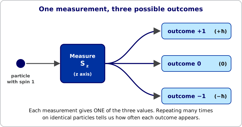 ![Measuring the spin along the z axis gives one of three outcomes: −1, 0 or +1 (in units of ħ).](../../img/sp-spin-outcomes.svg){fig-alt="A spin-1 particle enters a device that measures spin along the z axis. The beam splits into three possible outcomes: plus 1, 0 and minus 1, in units of h-bar." width="85%" fig-align="center"} A finite matrix is an approximation of the continuous position and momentum operators, so this model illustrates the ideas without reproducing the full theory. ## The data The matrices $S_x$, $S_y$, and $S_z$ are the spin components along the three axes. The matrix `C` is a second observable that shares the eigenvectors of $S_z$, which gives you a compatible pair to compare with the incompatible pair $S_x$ and $S_z$. The vector `state` is the first basis state: it has a definite value of $S_z$. ```{python} import matplotlib.pyplot as plt import numpy as np sqrt2 = np.sqrt(2) S_x = np.array([ [0, 1, 0], [1, 0, 1], [0, 1, 0] ], dtype=complex) / sqrt2 S_y = np.array([ [0, -1j, 0], [1j, 0, -1j], [0, 1j, 0] ], dtype=complex) / sqrt2 S_z = np.diag([1, 0, -1]).astype(complex) # A second observable that shares the eigenvectors of S_z. C = np.diag([2, 0, -2]).astype(complex) state = np.array([1, 0, 0], dtype=complex) print("S_x shape:", S_x.shape) print("State norm:", np.linalg.norm(state)) ``` For complex vectors and matrices, use the conjugate transpose, `.conj().T`, and not just `.T`, when you form inner products. The `@` operator performs matrix multiplication. Use the exact function names and parameters described below. Your functions must return their results; they should not print messages. ## Step 1: Check whether a matrix is Hermitian Create `is_hermitian(operator, tol=1e-10)`. 1. Compare the operator with its conjugate transpose. 2. Allow a small numerical tolerance, since floating-point calculations introduce tiny rounding differences. `np.allclose` is useful here. 3. Return a Boolean value. Use it to check the four supplied operators. Also try a small matrix that is not Hermitian, such as `[[0, 1], [0, 0]]`, and confirm that your function rejects it. ## Step 2: Find the possible measurement outcomes Create `get_eigensystem(operator)`. 1. Obtain the eigenvalues and eigenvectors of a Hermitian operator. `np.linalg.eigh` is designed for this case and returns the eigenvalues in increasing order. 2. Return the eigenvalues and a matrix whose **columns** are the corresponding eigenvectors. 3. Check that each eigenvector has unit length and that the eigenvectors are orthogonal. Hint: for the eigenvector matrix `V`, what should `V.conj().T @ V` be? 4. Check the action of the operator on all the eigenvectors at once: `operator @ V` should equal `V` with each column multiplied by its eigenvalue. Broadcasting the row of eigenvalues across the columns does this without a loop. The eigenvalues are the possible outcomes of a measurement. Rounding errors may show an eigenvalue as `-2.4e-16` instead of `0`; use `np.round` or `np.allclose` when you compare. For $S_x$ you should find the outcomes $-1$, $0$, and $1$. ## Step 3: Check whether two observables are compatible Create `commutator(A, B)` and `are_compatible(A, B, tol=1e-10)`. The commutator measures whether the order of two matrix products matters: $$ [A,B] = AB - BA. $$ 1. Compute the commutator using matrix multiplication. 2. Treat the operators as compatible when the commutator is close to the zero matrix, within the tolerance. 3. Check the pair $S_z$ and $C$, and then the pair $S_x$ and $S_z$. The first pair should be compatible and the second should not. 4. Use the eigenvectors from Step 2 to inspect whether the compatible pair has a shared eigenbasis. For Hermitian matrices, commuting operators can be described with a common orthonormal eigenbasis. Here the eigenvalues are all different, so you can compare the two bases directly. Eigenvectors may differ by a sign or a complex phase, so compare the **magnitude** of their inner products rather than their entries: for a shared basis, the matrix `np.abs(V1.conj().T @ V2)` is the identity matrix, up to the order of the columns. Compatibility means the two observables can have a shared set of definite states. Incompatibility means there is no common eigenbasis for the pair. ## Step 4: Calculate expectation and uncertainty Create `expectation_and_uncertainty(operator, state)`. For a normalized state vector $\psi$, the expectation value is $$ \langle A\rangle = \psi^\dagger A\psi, $$ and the uncertainty is the standard deviation of the possible outcomes: $$ \Delta A = \sqrt{\langle A^2\rangle - \langle A\rangle^2}. $$ 1. Use the conjugate transpose of the state when you compute the inner products. 2. Return the expectation value and the uncertainty as real numbers. 3. Floating-point rounding can make a variance that should be zero slightly negative. Avoid taking the square root of a negative number. Calculate the expectation and uncertainty of each supplied operator for `state`. You should find that $\Delta S_z = 0$ and $\Delta S_x = \Delta S_y = 1/\sqrt{2} \approx 0.71$. The state has a definite value of $S_z$ and an uncertain value of $S_x$ and $S_y$. For Hermitian observables $A$ and $B$, the general uncertainty relation is $$ \Delta A\,\Delta B \geq \frac{1}{2}\left|\langle [A,B]\rangle\right|. $$ This form connects the uncertainty to the commutator. The familiar $\hbar/2$ bound applies only to position and momentum; other pairs of observables have a different bound. Check this relation for $S_x$ and $S_y$ with `state`. Both sides should be $0.5$. ## Step 5: Simulate repeated measurements Create `simulate_measurements(operator, state, n_shots, rng)`. For a normalized state, the probability of observing the eigenvalue $i$ is the squared magnitude of the projection of the state onto the corresponding eigenvector: $$ p_i = |\mathbf{v}_i^\dagger\psi|^2. $$ 1. Find the eigenvalues and eigenvectors of the operator. 2. Calculate the probability of each outcome from the overlaps with the state. All of them at once: `V.conj().T @ state`. 3. Use `rng.choice` to draw `n_shots` outcomes with those probabilities. 4. Return the outcomes as a NumPy array. Use `rng = np.random.default_rng(42)` to make your experiment reproducible. Simulate measurements of $S_x$ and $S_z$ on many identically prepared copies of `state`. Compare the sample mean and standard deviation with the values from Step 4. A finite simulation fluctuates, but the estimates get closer to the theoretical values as you increase the number of shots. Use this plotting helper to display how often each outcome appears. You do not need to recreate or explain its code. ```{python} def plot_measurements(outcomes, label): values, counts = np.unique(outcomes, return_counts=True) fig, ax = plt.subplots() ax.bar(values, counts, width=0.6, color="#4472C4", edgecolor="white") ax.set_xlabel("Measurement outcome") ax.set_ylabel("Number of observations") ax.set_title(label) ax.set_xticks(values) ax.grid(axis="y", alpha=0.25) plt.show() plt.close(fig) ``` ## Step 6: Test and explain your model Run your functions on the supplied operators and state, and then design at least two tests of your own. For each test, write down the expected result before running your code. Check that: - All supplied observables are Hermitian, and the non-Hermitian test matrix is rejected. - The eigenvalues are real, and the eigenvectors form an orthonormal basis. - $S_z$ and $C$ are compatible, while $S_x$ and $S_z$ are not. - The chosen state has zero uncertainty in $S_z$ and nonzero uncertainty in $S_x$ and $S_y$. - For $S_x$ and $S_y$, the product of the uncertainties satisfies the general uncertainty relation. - Simulated averages and spreads are reasonably close to the theoretical values, and a measurement of $S_z$ on `state` always gives the same outcome. Then explain in your own words: 1. Why an eigenstate gives a definite outcome for its operator. 2. How the commutator relates to compatibility. 3. Why a finite simulation does not reproduce every possible measurement exactly. 4. What this finite model can show, and what it does not represent. ## Stretch goals (optional) 1. Prepare the state $|+x\rangle = (1/2,\ 1/\sqrt{2},\ 1/2)$ and repeat Steps 4 and 5. Which operator has now zero uncertainty? 2. Plot the estimated uncertainty of $S_x$ as a function of the number of shots, on a logarithmic axis, and describe how fast it approaches the theoretical value. 3. Build a random Hermitian matrix as `M + M.conj().T` for a random complex `M`, and verify that your functions work on it. ## Before you submit Upload your completed notebook to the **Side Projects** section on Blackboard **before the final exam**. Include your functions, your tests with saved outputs, the measurement plots, and your written explanations. Follow the notebook and AI-use guidance on the [Side Projects page](../structures/side_projects.qmd).