Flow and Congestion
Density Sweeps and Fundamental Diagrams
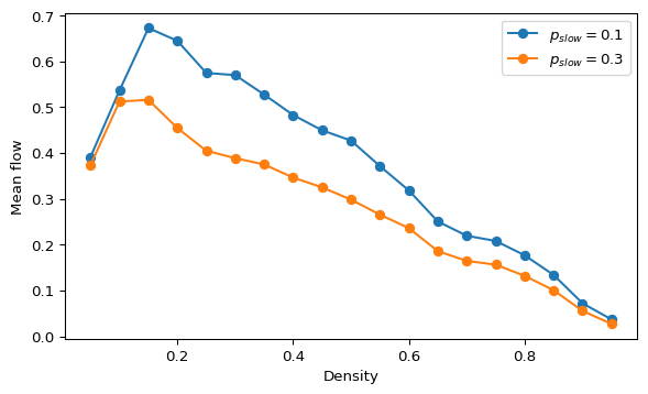
Once the simulator works, the next step is to extract macroscopic observables. In traffic modeling the most important one is the fundamental diagram, the relationship between density and average flow (Nagel and Schreckenberg 1992).
Measure density and flow
Two standard macroscopic quantities are
\[ \rho = \frac{N_{\mathrm{cars}}}{L}, \qquad q(t) = \frac{1}{L}\sum_{i \in \mathrm{cars}} v_i(t). \]
Here \(\rho\) is the density and \(q(t)\) is the instantaneous flow, measured as the mean number of cells traveled per road cell and per time step.
To estimate stationary behavior, average \(q(t)\) after a burn-in window.
Record flow during one run
The simplest extension of the simulator is to track the flow after each update.
def simulate_with_flow(steps, length, density, vmax, p_slow, seed):
    rng = np.random.default_rng(seed)
    occupied, speeds = initialize_road(length=length, density=density, vmax=vmax, rng=rng)

    flow_history = np.zeros(steps)
    flow_history[0] = speeds[occupied].sum() / length

    for t in range(1, steps):
        occupied, speeds = step(
            occupied,
            speeds,
            vmax=vmax,
            p_slow=p_slow,
            rng=rng,
        )
        flow_history[t] = speeds[occupied].sum() / length

    return flow_history
Sweep the density
Now repeat the experiment for many densities.
densities = np.linspace(0.05, 0.95, 19)
mean_flows = []

for density in densities:
    flow_history = simulate_with_flow(
        steps=300,
        length=100,
        density=density,
        vmax=5,
        p_slow=0.3,
        seed=7,
    )
    mean_flows.append(flow_history[100:].mean())
Plotting mean_flows against densities gives the fundamental diagram.
Compare slowdown probabilities
The most informative parameter to vary is p_slow.
- At small density, cars rarely interact and the flow grows roughly linearly with density.
- At intermediate density, the flow reaches a maximum.
- At high density, braking dominates and the flow drops because congestion limits motion.
Increasing p_slow usually lowers the peak flow and shifts the congested regime earlier.
Practical tip
Use several seeds if you want smoother curves. For example, estimate the mean flow for each density with 5 to 10 trials and then average the stationary values.
What to Report
- A space-time diagram in a free-flow regime.
- A space-time diagram in a congested regime.
- At least one flow-density curve.
- A short interpretation of where the maximum flow occurs and how noise changes it.
What’s Next?
You now have both scales of the model: the microscopic update and the macroscopic observables. The assignment combines them into one coherent traffic study.
References
Nagel, Kai, and Michael Schreckenberg. 1992. “A Cellular Automaton Model for Freeway Traffic.” Journal de Physique I 2 (12): 2221–29. https://doi.org/10.1051/jp1:1992277.