Rule Exploration

Comparing Rules and Initial Conditions

Once one simulator works, the interesting question is no longer “can I update the row?” but “what changes when only the local rule changes?” This is where cellular automata become a modeling lab rather than a single example.

Figure 1: Four elementary rules started from the same single-seed initial condition.

Build a reusable simulator

The core function should take three inputs: an initial row, a rule number, and the number of time steps.

def simulate_ca(initial_state, rule_number, steps):
    rule_bin = np.array([int(bit) for bit in f"{rule_number:08b}"])
    grid = np.zeros((steps, len(initial_state)), dtype=int)
    grid[0] = initial_state

    for t in range(1, steps):
        grid[t] = apply_rule(grid[t - 1], rule_bin)

    return grid

With this wrapper in place, changing the experiment only means changing the inputs.

Compare several rules

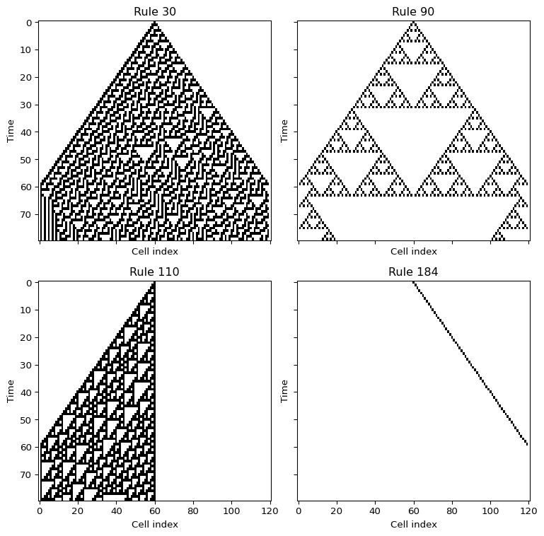
Rules 30, 90, 110, and 184 are a good first comparison because they already show very different behavior.

• Rule 90 creates a highly regular, symmetric pattern.
• Rule 30 quickly becomes irregular and looks almost random.
• Rule 110 shows localized structures and interacting motifs.
• Rule 184 transports occupied sites to the right and is a useful bridge to traffic models.

rules = [30, 90, 110, 184]

for rule_number in rules:
    grid = simulate_ca(initial_state, rule_number, steps=80)
    plt.figure(figsize=(6, 4))
    plt.imshow(grid, cmap="binary", interpolation="nearest", aspect="auto")
    plt.title(f"Rule {rule_number}")
    plt.xlabel("Cell index")
    plt.ylabel("Time")
    plt.show()

Change the initial condition

The second important experiment is to keep the rule fixed and change only the first row.

rng = np.random.default_rng(7)
initial_state = (rng.random(121) < 0.5).astype(int)

grid = simulate_ca(initial_state, rule_number=110, steps=80)
plt.imshow(grid, cmap="binary", interpolation="nearest", aspect="auto")
plt.show()

This lets you separate two effects:

• what is imposed by the rule itself,
• and what is inherited from the initial data.

Optional stochastic extension

If you want to go one step further, add noise after each update. For example, flip each cell with a small probability p_flip.

def noisy_update(state, rule_bin, p_flip=0.01, rng=None):
    if rng is None:
        rng = np.random.default_rng()

    new_state = apply_rule(state, rule_bin)
    flips = rng.random(len(new_state)) < p_flip
    new_state[flips] = 1 - new_state[flips]
    return new_state

That changes the model from a deterministic rule system into a stochastic one.

Questions for Your Notes

• Which rule preserves symmetry most clearly?
• Which rule seems most sensitive to tiny changes in the first row?
• Which rule looks most like transport or directed motion?

What’s Next?

Rule 184 is already a useful bridge to traffic because occupied cells move to the right under a local exclusion rule. In the next session we keep that traffic intuition, but each car gets its own speed and a random braking rule.

Assignment Next Session: Agent-Based Modeling