Gierer-Meinhardt Model in 2D
Extending the Solver to a Grid
Now we lift the same reaction terms to two spatial dimensions. The main conceptual change is the Laplacian. Everything else follows the same workflow you already used in 1D.
If your 1D code was modular, half the work is already done. This page is mostly about changing the data shape and handling neighbors in two directions instead of one.
The PDE is still
\[ \begin{aligned} \frac{\partial u}{\partial t} &= \Delta u + \gamma \left(a - b u + \frac{u^2}{v}\right), \\ \frac{\partial v}{\partial t} &= d\,\Delta v + \gamma \left(u^2 - v\right), \end{aligned} \tag{1}\]
but now \(u\) and \(v\) depend on \((x, y, t)\).
Rectangular Domains in Cartesian Coordinates
We work on a rectangle \([0, L_x] \times [0, L_y]\). After discretization, each field becomes a matrix.
- The row index stores the \(x\) position.
- The column index stores the \(y\) position.
- The full state has shape
(2, num_x, num_y)because we track both \(u\) and \(v\).
With a common grid spacing \(dx\), we use
num_x = int(length_x / dx)
num_y = int(length_y / dx)
uv = np.ones((2, num_x, num_y))
The important numerical point is that we still update the whole matrix at once. We do not loop over grid points one by one. We shift the full matrix up, down, left, and right, then combine those shifted copies in a vectorized stencil.
Discretize the 2D Laplacian
This is the real jump from the previous page. In 1D, every point had two nearest neighbors. In 2D, every point in the interior has four cardinal neighbors, so the Laplacian becomes a stencil on a grid.
In two dimensions,
\[ \Delta u = \frac{\partial^2 u}{\partial x^2} + \frac{\partial^2 u}{\partial y^2}. \tag{2}\]
The standard 5-point stencil is
\[ \Delta u(x,y) \approx \frac{u(x+dx,y) + u(x-dx,y) + u(x,y+dx) + u(x,y-dx) - 4u(x,y)}{dx^2}. \tag{3}\]
Implement that stencil with np.roll(). Each np.roll() call shifts the whole matrix by one grid cell along one Cartesian direction.
import numpy as np

def laplacian_2d(field, dx):
    # TODO: combine the four nearest neighbors and the center point
    lap =
    return lap / dx**2
Hint: 2D Laplacian (click to expand)
def laplacian_2d(field, dx):
    lap = -4 * field
    lap += np.roll(field, shift=1, axis=0)
    lap += np.roll(field, shift=-1, axis=0)
    lap += np.roll(field, shift=1, axis=1)
    lap += np.roll(field, shift=-1, axis=1)
    return lap / dx**2
Note
This stencil uses matrix shifts, so the same helper works for every boundary condition. The difference comes after the Euler step, when you decide whether to wrap, copy, or pin the edges.
Boundary Conditions on a Rectangle
On a rectangle, boundary conditions are enforced on the four edges. The implementation pattern is always the same.
- Periodic: leave the array unchanged after the Euler step because
np.roll()already wraps one side onto the opposite side. - Neumann: copy the nearest interior row or column onto the boundary, which sets the normal derivative to zero.
- Dirichlet: overwrite the boundary with prescribed values after each Euler step.
def apply_boundary_conditions(uv, bc="neumann", dirichlet_values=(1.0, 1.0)):
    if bc == "periodic":
        return uv

    if bc == "neumann":
        uv[:, 0, :] = uv[:, 1, :]
        uv[:, -1, :] = uv[:, -2, :]
        uv[:, :, 0] = uv[:, :, 1]
        uv[:, :, -1] = uv[:, :, -2]
        return uv

    if bc == "dirichlet":
        u_bc, v_bc = dirichlet_values
        uv[0, 0, :] = u_bc
        uv[0, -1, :] = u_bc
        uv[0, :, 0] = u_bc
        uv[0, :, -1] = u_bc
        uv[1, 0, :] = v_bc
        uv[1, -1, :] = v_bc
        uv[1, :, 0] = v_bc
        uv[1, :, -1] = v_bc
        return uv

    raise ValueError("bc must be 'periodic', 'neumann', or 'dirichlet'")
For the Gierer-Meinhardt examples on this page, we keep Neumann boundaries. On the Gray-Scott page, we will keep the exact same Laplacian and Euler loop but switch the interpretation to periodic boundaries.
Initialize the Grid
import numpy as np

np.random.seed(3)

length_x = 20
length_y = 50
dx = 1
num_x = int(length_x / dx)
num_y = int(length_y / dx)

# TODO: create a homogeneous state with u = 1 and v = 1
uv =

# TODO: add 1% random perturbations
uv +=
Hint: 2D initialization (click to expand)
uv = np.ones((2, num_x, num_y))
uv += uv * np.random.randn(2, num_x, num_y) / 100
Build the PDE Right-Hand Side
def gierer_meinhardt_pde_2d(t, uv, gamma=1, a=0.40, b=1.00, d=20, dx=1):
    u, v = uv
    lu = laplacian_2d(u, dx)
    lv = laplacian_2d(v, dx)

    # TODO: write the reaction terms
    f =
    g =

    # TODO: combine diffusion and reaction
    du_dt =
    dv_dt =
    return np.array([du_dt, dv_dt])
Hint: Gierer-Meinhardt PDE in 2D (click to expand)
def gierer_meinhardt_pde_2d(t, uv, gamma=1, a=0.40, b=1.00, d=20, dx=1):
    u, v = uv
    lu = laplacian_2d(u, dx)
    lv = laplacian_2d(v, dx)

    f = a - b * u + (u**2) / v
    g = u**2 - v
    du_dt = lu + gamma * f
    dv_dt = d * lv + gamma * g
    return np.array([du_dt, dv_dt])
Write the Euler Step Once
Once the right-hand side is available, the full PDE update is just explicit Euler applied to the whole tensor:
\[ UV^{n+1} = UV^n + dt\,G(UV^n). \]
In code, that means one vectorized update followed by one boundary-condition update.
dudt, dvdt = gierer_meinhardt_pde_2d(0, uv, dx=dx)
uv[0] = uv[0] + dt * dudt
uv[1] = uv[1] + dt * dvdt
uv = apply_boundary_conditions(uv, bc="neumann")
The order matters. First compute the Euler step, then reapply the edge values so the next stencil evaluation sees data consistent with the chosen boundary condition.
Time Step with Euler’s Method
Before you animate anything, validate the numerical update with a long loop and one static snapshot. That is the same workflow we used in earlier sessions: get the update rule right first, then wrap it in animation logic.
num_iter = 50000
dt = 0.001

for _ in range(num_iter):
    dudt, dvdt = gierer_meinhardt_pde_2d(0, uv, dx=dx)

    # TODO: Euler update for u and v

    # TODO: reapply Neumann boundary conditions on the rectangle
Hint: 2D Euler loop (click to expand)
for _ in range(num_iter):
dudt, dvdt = gierer_meinhardt_pde_2d(0, uv, dx=dx)
uv[0] = uv[0] + dt * dudt
uv[1] = uv[1] + dt * dvdt
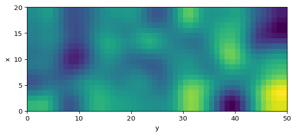
uv = apply_boundary_conditions(uv, bc="neumann")Plot a Snapshot
import matplotlib.pyplot as plt

fig, ax = plt.subplots(figsize=(7, 4))
im = ax.imshow(
    uv[1],
    interpolation="bilinear",
    origin="lower",
    extent=[0, length_y, 0, length_x],
)
ax.set_xlabel("y")
ax.set_ylabel("x")
plt.colorbar(im, ax=ax, label="v(x, y)")
plt.show()
Animate the Simulation
import matplotlib.animation as animation
import matplotlib.pyplot as plt

fig, ax = plt.subplots(figsize=(7, 4))
im = ax.imshow(uv[1], origin="lower", extent=[0, length_y, 0, length_x])

def update_frame(_):
    # TODO: advance uv by one or several Euler steps
    # TODO: reapply Neumann boundary conditions
    im.set_array(uv[1])
    return (im,)

ani = animation.FuncAnimation(fig, update_frame, interval=1, blit=True)
Hint: 2D animation update (click to expand)
def update_frame(_):
    nonlocal uv
    dudt, dvdt = gierer_meinhardt_pde_2d(0, uv, dx=dx)
    uv[0] = uv[0] + dt * dudt
    uv[1] = uv[1] + dt * dvdt
    uv = apply_boundary_conditions(uv, bc="neumann")
    im.set_array(uv[1])
    return (im,)
Optional: Try a 9-Point Stencil
The 5-point stencil is the standard choice, but you can improve the rotational symmetry of the Laplacian with a 9-point stencil. That is a good extension if you want to compare numerical accuracy.
Explore
Use the Turing page to compare the cases \(d=20\) and \(d=30\). Does the pattern that forms on your grid match the change suggested by the unstable mode analysis?
What’s Next?
The Gierer-Meinhardt model is a good training ground, but the final target of the session is Gray-Scott. It uses the same numerical ideas with different reaction terms and richer visual patterns.
Tip
Reference code is available in amlab/pdes/gierer_meinhardt_2d.py.