Sensitivity and Chaos
Nearby Trajectories and Predictability
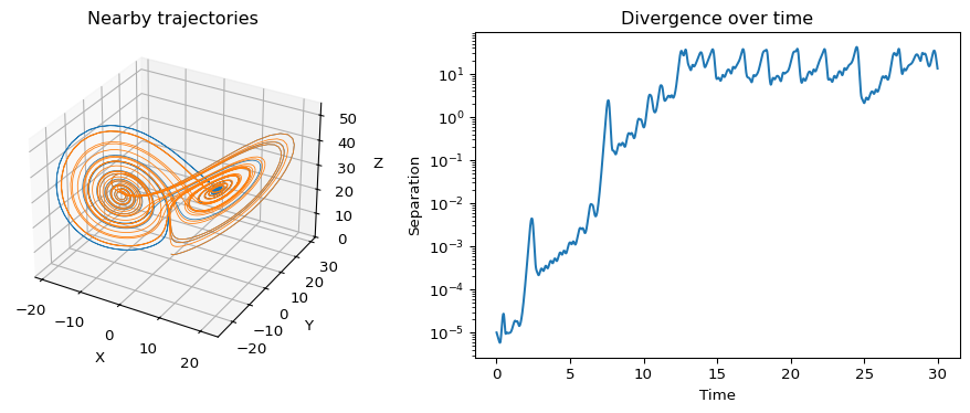
The Lorenz attractor is deterministic, but long-term prediction is still limited because nearby trajectories diverge over time (Lorenz 1963; Strogatz 2024). This is the signature feature of sensitivity to initial conditions.
Compare two nearby initial conditions
To test sensitivity, keep the parameters fixed and change only the initial state by a tiny amount.
initial_state_a = (0.0, 1.0, 1.05)
initial_state_b = (0.0, 1.0, 1.05001)

trajectory_a = simulate_lorenz(initial_state=initial_state_a, dt=0.01, num_steps=3000)
trajectory_b = simulate_lorenz(initial_state=initial_state_b, dt=0.01, num_steps=3000)
At first, the two runs are nearly indistinguishable. Later, they separate enough that their detailed future motion no longer matches.
Measure the separation
The most direct diagnostic is the Euclidean distance between the two trajectories at each time step:
\[ d_n = \left\|\mathbf{x}_n^{(1)} - \mathbf{x}_n^{(2)}\right\|. \]
separation = np.linalg.norm(trajectory_a - trajectory_b, axis=1)
times = 0.01 * np.arange(len(separation))

plt.semilogy(times, separation)
plt.xlabel("Time")
plt.ylabel("Separation")
plt.show()
If the separation grows rapidly from a tiny initial perturbation, then the predictability horizon is short even though the equations themselves are deterministic.
What chaos means here
In this context, chaos does not mean that the model is random.
- The update rule is fixed.
- The same initial condition gives the same trajectory.
- Small errors in the initial state can still lead to very different long-run outcomes.
This is why deterministic chaos matters in modeling. Exact equations do not guarantee exact long-term forecasts.
Parameter variation
The parameter r strongly influences the geometry of the trajectories. A useful first comparison is to simulate one run with a smaller value such as r=10 and another with the standard value r=28.
trajectory_low_r = simulate_lorenz(dt=0.01, num_steps=3000, r=10)
trajectory_standard = simulate_lorenz(dt=0.01, num_steps=3000, r=28)
That comparison helps separate two ideas:
- sensitivity to initial conditions at fixed parameters,
- and qualitative changes driven by the parameter regime.
What’s Next?
The assignment combines the geometric picture of the attractor with the quantitative evidence for sensitivity to initial conditions.
References
Lorenz, Edward N. 1963. “Deterministic Nonperiodic Flow.” Journal of the Atmospheric Sciences 20 (2): 130–41. https://doi.org/10.1175/1520-0469(1963)020<0130:DNF>2.0.CO;2.
Strogatz, Steven H. 2024. Nonlinear Dynamics and Chaos: With Applications to Physics, Biology, Chemistry, and Engineering. Chapman; Hall/CRC.