Gierer-Meinhardt Model in 1D
Your First Reaction-Diffusion PDE
The Gierer-Meinhardt model is a classical activator-inhibitor system that produces spatial patterns when diffusion and reaction act together (Gierer and Meinhardt 1972). We will use it to learn the full PDE workflow in one space dimension.
In the ODE sessions, the state was a short vector and solve_ivp() took care of the time integration. Here the state is a field sampled on a grid, so we must build the update rule ourselves. The logic is still familiar: define the right-hand side, choose parameters, advance in time, and visualize the result.
The model reads
\[ \begin{aligned} \frac{\partial u}{\partial t} &= \Delta u + \gamma \left(a - b u + \frac{u^2}{v}\right), \\ \frac{\partial v}{\partial t} &= d\,\Delta v + \gamma \left(u^2 - v\right), \end{aligned} \tag{1}\]
where \(u(x,t)\) is the activator, \(v(x,t)\) is the inhibitor, and \(d\) is the diffusion ratio of \(v\).
Read the Parameters First
Before you discretize the PDE, it helps to know what each symbol controls.
- \(u(x,t)\) is the activator. Through the term \(u^2 / v\), a local increase in \(u\) tends to reinforce further production of \(u\).
- \(v(x,t)\) is the inhibitor. It suppresses activation because larger \(v\) reduces the ratio \(u^2 / v\).
- \(a\) is a baseline source term for \(u\). Larger \(a\) raises the background activity level.
- \(b\) damps the activator linearly. Larger \(b\) makes it harder for \(u\) to remain large.
- \(\gamma\) sets the reaction timescale. Larger \(\gamma\) makes the reaction terms act faster relative to diffusion.
- \(d\) is the diffusion ratio of the inhibitor. In this nondimensional form, \(u\) diffuses with coefficient \(1\), so large \(d\) means that \(v\) spreads much faster than \(u\).
The homogeneous steady state is
\[ u_* = \frac{a+1}{b}, \qquad v_* = \left(\frac{a+1}{b}\right)^2. \tag{2}\]
This is the flat state that we later test for pattern formation.
The short picture is this: the activator tends to build local peaks, while the inhibitor spreads the suppressing signal over a wider region.
What Instability Means Here
The phrase “Turing instability” has a very specific meaning. It does not mean the model explodes or becomes unstable in every possible way. It means the flat steady state is stable to spatially uniform perturbations, but unstable to some spatially varying ones.
In practice, this means two things.
- If every point is nudged in the same way, the system relaxes back toward the steady state.
- If one region is nudged slightly above its neighbors, that spatial difference can grow into a visible pattern.
This is why the model is interesting. Diffusion does not only smooth the field. For suitable reaction parameters, a fast-diffusing inhibitor can make a subset of spatial perturbations grow instead of decay.
Does no Turing instability mean that the inhibitor dominates?
Not necessarily. It means that the system is not in the right regime for diffusion-driven pattern formation.
There are several ways this can happen.
- The inhibitor may be too strong, so spatial bumps are suppressed.
- The activator may be too weak to reinforce a local perturbation.
- The inhibitor may fail to diffuse fast enough relative to the activator.
- The homogeneous steady state may already be unstable for reasons unrelated to the Turing mechanism.
The safest summary is this: no Turing instability does not mean that one species simply “wins.” It means that the balance between local activation, inhibition, and diffusion does not selectively amplify spatial modes.
The next page, Turing Instability, turns this intuition into algebra and gives the inequalities that define the instability region.
What the Modes Mean
The instability does not amplify every spatial perturbation equally. On a finite domain with fixed boundary conditions, only certain spatial shapes are natural building blocks. These are the modes.
For Neumann boundary conditions on \([0,L]\), the admissible 1D modes are proportional to
\[ \cos\left(\frac{n\pi x}{L}\right), \qquad n = 0, 1, 2, \dots \tag{3}\]
These mode numbers have a simple interpretation as spatial frequencies.
- Mode \(0\) is flat, with no spatial variation.
- Mode \(1\) has the longest non-constant wavelength allowed by the domain.
- Mode \(2\) oscillates twice as fast in space.
- Mode \(3\) oscillates three times as fast.
- Higher modes have shorter wavelengths and finer structure.
When we say a mode is unstable, we mean that a tiny perturbation with that spatial shape grows over time in the linearized system. The leading mode is the one with the largest growth rate, so it usually sets the early spacing of the pattern.
Later, the full nonlinear dynamics can merge peaks, saturate amplitudes, or shift the final profile. That is why the leading mode predicts the early pattern best, even if the long-time state looks different.
Discretize the Laplacian
In one dimension, the Laplacian is the second derivative:
\[ \Delta u = \frac{d^2 u}{dx^2}. \tag{4}\]
Using a centered finite difference with spacing \(dx\) gives
\[ \Delta u(x) \approx \frac{u(x+dx) - 2u(x) + u(x-dx)}{dx^2}. \tag{5}\]
Where does this formula come from?
The second derivative is the limit of the difference quotient:
\[ \frac{d^2 u}{dx^2} = \lim_{dx \to 0} \frac{u(x+dx) - 2u(x) + u(x-dx)}{dx^2}. \]
This is a direct consequence of the Taylor expansion of \(u\) around \(x\):
\[ \begin{aligned} u(x+dx) &= u(x) + u'(x) dx + \frac{1}{2} u''(x) dx^2 + \mathcal{O}(dx^3), \\ u(x-dx) &= u(x) - u'(x) dx + \frac{1}{2} u''(x) dx^2 + \mathcal{O}(dx^3). \end{aligned} \]
Adding these two expansions gives
\[ u(x+dx) + u(x-dx) = 2u(x) + u''(x) dx^2 + \mathcal{O}(dx^3), \]
which can be rearranged to give the finite difference formula, ignoring the higher-order terms \(\mathcal{O}(dx^3)\).
Write a helper that computes this second derivative for a 1D field.
import numpy as np

def laplacian_1d(values, dx):
    # TODO: use the left and right neighbors of each grid point
    lap =
    return lap / dx**2
Hint: 1D Laplacian (click to expand)
def laplacian_1d(values, dx):
    lap = -2 * values
    lap += np.roll(values, shift=1)
    lap += np.roll(values, shift=-1)
    return lap / dx**2
Choose Boundary Conditions
We need one more ingredient before we time step the PDE: what happens at the edges of the domain?
In previous sessions, the numerical solver handled most of the bookkeeping for us. In PDEs, boundary conditions are part of the model, so we must enforce them by hand after every update.
Neumann boundary conditions
Zero flux means that the slope at the boundary is zero. Numerically, a simple implementation is to copy the nearest interior value:
\[ u(0) = u(dx), \qquad u(L) = u(L-dx). \tag{6}\]
Periodic boundary conditions
The left and right endpoints are identified. This is exactly what np.roll() assumes.
Dirichlet boundary conditions
You prescribe fixed values at the endpoints.
In this page we will use Neumann boundary conditions because they are easy to interpret in a chemical setting.
Initialize the Fields
Start from the homogeneous state and add a small perturbation.
import numpy as np

np.random.seed(3)

length = 40
dx = 0.5
num_points = int(length / dx)

# TODO: create a (2, num_points) array filled with ones
uv =

# TODO: add 1% Gaussian noise to break symmetry
uv +=
Hint: Field initialization (click to expand)
uv = np.ones((2, num_points))
uv += uv * np.random.randn(2, num_points) / 100
Why do we add noise? A perfectly uniform initial condition can hide an instability. Small perturbations reveal whether the system amplifies spatial differences.
Build the PDE Right-Hand Side
Use your Laplacian helper for both \(u\) and \(v\), then add the reaction terms.
def gierer_meinhardt_pde(t, uv, gamma=1, a=0.40, b=1.00, d=20, dx=0.5):
    u, v = uv
    lu = laplacian_1d(u, dx)
    lv = laplacian_1d(v, dx)

    # TODO: write the reaction terms
    f =
    g =

    # TODO: combine diffusion and reaction
    du_dt =
    dv_dt =
    return np.array([du_dt, dv_dt])
Hint: Gierer-Meinhardt PDE in 1D (click to expand)
def gierer_meinhardt_pde(t, uv, gamma=1, a=0.40, b=1.00, d=20, dx=0.5):
    u, v = uv
    lu = laplacian_1d(u, dx)
    lv = laplacian_1d(v, dx)

    f = a - b * u + (u**2) / v
    g = u**2 - v
    du_dt = lu + gamma * f
    dv_dt = d * lv + gamma * g
    return np.array([du_dt, dv_dt])
Advance in Time
We will use explicit Euler:
\[ u^{n+1} = u^n + dt\,\dot u^n, \qquad v^{n+1} = v^n + dt\,\dot v^n. \tag{7}\]
Complete the loop below.
num_iter = 50000
dt = 0.001

for _ in range(num_iter):
    dudt, dvdt = gierer_meinhardt_pde(0, uv, dx=dx)

    # TODO: Euler update for u and v

    # TODO: Neumann boundary conditions on both fields
Hint: Euler loop with Neumann boundaries (click to expand)
for _ in range(num_iter):
dudt, dvdt = gierer_meinhardt_pde(0, uv, dx=dx)
uv[0] = uv[0] + dt * dudt
uv[1] = uv[1] + dt * dvdt
uv[:, 0] = uv[:, 1]
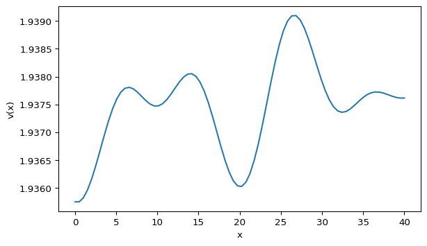
uv[:, -1] = uv[:, -2]Plot the Pattern
import matplotlib.pyplot as plt
import numpy as np

x = np.linspace(0, length, num_points)
fig, ax = plt.subplots(figsize=(7, 4))
ax.plot(x, uv[1])
ax.set_xlabel("x")
ax.set_ylabel("v(x)")
ax.set_title("Gierer-Meinhardt in 1D")
plt.show()
Your profile should look qualitatively similar to Figure 1. The exact peak locations will differ because the initial noise is random.
Animation Extension
As in the animation pages from the previous sessions, once the update rule works in a loop, the animation is mostly a matter of moving that loop into a Matplotlib callback.
Move the Euler update inside a Matplotlib animation callback.
import matplotlib.animation as animation
import matplotlib.pyplot as plt

fig, ax = plt.subplots(figsize=(7, 4))
(plot_v,) = ax.plot(x, uv[1])
ax.set_xlabel("x")
ax.set_ylabel("v(x)")

def update_frame(_):
    # TODO: advance uv by one Euler step
    # TODO: update the line data
    return (plot_v,)

ani = animation.FuncAnimation(fig, update_frame, interval=1, blit=True)
Hint: 1D animation update (click to expand)
def update_frame(_):
    nonlocal uv
    dudt, dvdt = gierer_meinhardt_pde(0, uv, dx=dx)
    uv[0] = uv[0] + dt * dudt
    uv[1] = uv[1] + dt * dvdt
    uv[:, 0] = uv[:, 1]
    uv[:, -1] = uv[:, -2]
    plot_v.set_data(x, uv[1])
    return (plot_v,)
Explore
Try \(d=30\) instead of \(d=20\). Do the peaks become sharper, flatter, or more numerous? On the next page we will use Turing instability to explain why some parameter choices create patterns and others do not.
What’s Next?
You now have a working 1D solver. The next question is theoretical: for which parameter values should the uniform state break and form a pattern?
Tip
Reference code is available in amlab/pdes/gierer_meinhardt_1d.py.
References
Gierer, Alfred, and Hans Meinhardt. 1972. “A Theory of Biological Pattern Formation.” Kybernetik 12 (1): 30–39. https://doi.org/10.1007/BF00289234.