import matplotlib.pyplot as plt
import networkx as nx

SEED = 7


def summarize_graph(G, name="G"):
    """Print a small summary table of common network statistics."""
    n = G.number_of_nodes()
    m = G.number_of_edges()
    avg_k = 2 * m / n if n > 0 else 0
    density = nx.density(G)

    # Connectivity (undirected)
    is_connected = nx.is_connected(G) if n > 0 else False
    n_components = nx.number_connected_components(G) if n > 0 else 0

    # Work on largest connected component when disconnected
    if n == 0:
        L = float("nan")
        C = float("nan")
    else:
        C = nx.average_clustering(G)
        if is_connected:
            L = nx.average_shortest_path_length(G)
        else:
            largest_cc = max(nx.connected_components(G), key=len)
            H = G.subgraph(largest_cc).copy()
            L = nx.average_shortest_path_length(H)

    print(f"--- {name} ---")
    print(f"N = {n}, E = {m}, <k> = {avg_k:.2f}, density = {density:.4f}")
    print(f"connected = {is_connected}, components = {n_components}")
    print(f"clustering C = {C:.3f}")
    print(f"avg shortest path L = {L:.3f} (largest CC if disconnected)")


def plot_degree_histogram(G, title="Degree distribution"):
    degrees = [deg for _, deg in G.degree()]
    plt.figure(figsize=(5, 3))
    plt.hist(degrees, bins=range(min(degrees), max(degrees) + 2), align="left", rwidth=0.9)
    plt.xlabel("Degree k")
    plt.ylabel("Count")
    plt.title(title)
    plt.tight_layout()
plt.show()Networks: Graph Models
Random, Small-World, Scale-Free
Real networks (social, transportation, communication) are not arbitrary: they tend to have short paths, clustering, and sometimes hubs (Newman 2018).
In this page, we introduce three classic synthetic graph models that help us reproduce (some of) these properties:
- Random graphs (Erdős–Rényi / Gilbert)
- Small-world graphs (Watts–Strogatz)
- Scale-free graphs (Barabási–Albert preferential attachment)
We will also compute a few summary metrics for each model:
- Average degree \(\langle k \rangle\)
- Density \(D\)
- Average clustering coefficient \(C\)
- Average shortest path length \(L\) (on the largest connected component if needed)
If you have not seen these metrics before, the definitions and examples are in the previous page: Network Connectivity.
Random graphs (Erdos–Rényi / Gilbert)
In the Gilbert model \(G(N, p)\), we consider every possible pair of nodes and include the edge independently with probability \(p\) (Gilbert 1959; Erdos and Renyi 1959).
Key properties (typical, for large \(N\)):
- Degree distribution is approximately binomial, and approaches Poisson in the sparse limit.
- Average clustering is approximately \(C \approx p\).
- Typical path lengths scale like \(L \sim \log N\) when the graph is above the connectivity threshold.
In NetworkX, you can create this model with nx.erdos_renyi_graph(n, p) (alias: nx.gnp_random_graph).
- Select a pair of nodes, say i and j.
- Generate a random number r between 0 and 1. If r < p, then add a link between i and j.
- Repeat (1) and (2) for all pairs of nodes.
# Random graph G(N, p)
G_random = nx.erdos_renyi_graph(n=80, p=0.06, seed=SEED)

pos = nx.spring_layout(G_random, seed=SEED)
nx.draw(G_random, pos=pos, node_size=120, node_color="lightgray", edge_color="gray")
plt.title("Erdos–Rényi random graph")
plt.show()

summarize_graph(G_random, name="Random (G(N,p))")
plot_degree_histogram(G_random, title="Random graph: degree distribution")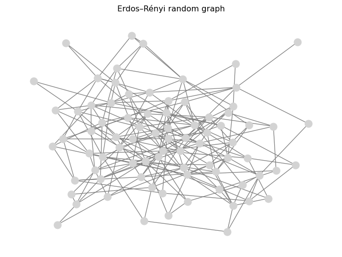
--- Random (G(N,p)) ---
N = 80, E = 211, <k> = 5.28, density = 0.0668
connected = True, components = 1
clustering C = 0.078
avg shortest path L = 2.766 (largest CC if disconnected)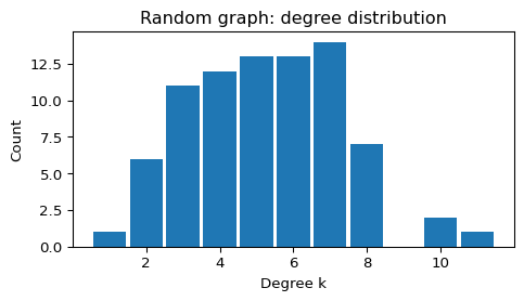
\(G(N, p)\) vs \(G(N, m)\)
Another popular variant is \(G(N, m)\), where we fix the number of edges \(m\) instead of an edge probability. In NetworkX:
nx.gnm_random_graph(n, m)implements \(G(N,m)\)nx.erdos_renyi_graph(n, p)implements \(G(N,p)\)
# Random graph G(N, m)
G_gnm = nx.gnm_random_graph(n=80, m=180, seed=SEED)
summarize_graph(G_gnm, name="Random (G(N,m))")
plot_degree_histogram(G_gnm, title="G(N,m): degree distribution")
--- Random (G(N,m)) ---
N = 80, E = 180, <k> = 4.50, density = 0.0570
connected = False, components = 2
clustering C = 0.039
avg shortest path L = 3.026 (largest CC if disconnected)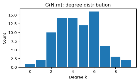
Small-world graphs (Watts–Strogatz)
Watts–Strogatz networks start from a ring lattice (high clustering, long paths) and then rewire edges with probability \(p\) (Watts and Strogatz 1998).
Key properties:
- For small \(p\) (e.g. \(p \in [0.01, 0.2]\)), you often get high clustering and short path lengths (“small-world”).
- Degree distribution stays relatively narrow (most nodes have degree near \(k\)).
In NetworkX:
nx.watts_strogatz_graph(n, k, p)generates the classic model.kis the number of neighbors of each node in the initial ring (typically even).
- Begin with a ring of \(N\) nodes
- Connect each node to its \(k\) nearest neighbors (or \(k-1\) if k is odd).
- For each edge \((u, v)\), with probability \(p\), replace edge \((u, v)\) with \((u, w)\) where \(w\) is not a neighbor of \(u\).
# Watts-Strogatz small-world graph with n nodes, k neighbors, and probability p of rewiring
G_sw = nx.watts_strogatz_graph(n=80, k=6, p=0.08, seed=SEED)

pos = nx.spring_layout(G_sw, seed=SEED)
nx.draw(G_sw, pos=pos, node_size=120, node_color="lightblue", edge_color="gray")
plt.title("Watts–Strogatz small-world graph")
plt.show()

summarize_graph(G_sw, name="Small-world (Watts–Strogatz)")
plot_degree_histogram(G_sw, title="Small-world: degree distribution")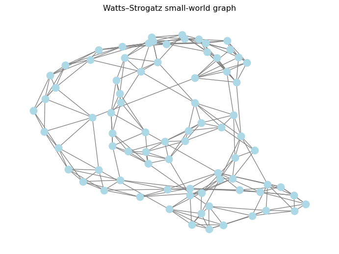
--- Small-world (Watts–Strogatz) ---
N = 80, E = 240, <k> = 6.00, density = 0.0759
connected = True, components = 1
clustering C = 0.494
avg shortest path L = 3.694 (largest CC if disconnected)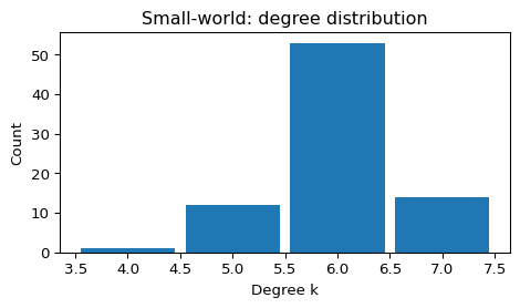
Scale-free graphs (preferential attachment)
Many real networks exhibit a heavy-tailed (sometimes approximately power-law) degree distribution: most nodes have small degree, but a few nodes become hubs (Barabasi and Albert 1999; Newman 2018).
The Barabási–Albert (BA) model generates this effect via preferential attachment (Barabasi and Albert 1999):
- Nodes that already have many edges are more likely to receive new edges.
Key properties (typical):
- Degree distribution is heavy-tailed (often summarized as “scale-free”).
- Small average path length (hubs create shortcuts).
- Clustering is usually lower than small-world models (but there are variants that increase clustering).
In NetworkX:
nx.barabasi_albert_graph(n, m)where each new node attaches tomexisting nodes.
- Start with a clique of \(m + 1\) nodes.
- Select \(m\) different nodes at random, weighted by their degree.
- Add a new node \(i\) and link it with the \(m\) nodes from the previous step.
- Repeat 2-3 until there are N nodes in the graph.
# Barabasi-Albert preferential attachment graph with n nodes and m edges
G_sf = nx.barabasi_albert_graph(n=200, m=2, seed=SEED)

pos = nx.spring_layout(G_sf, seed=SEED)
nx.draw(G_sf, pos=pos, node_size=35, node_color="lightgreen", edge_color="gray", alpha=0.8)
plt.title("Barabási–Albert (scale-free-ish) graph")
plt.show()

summarize_graph(G_sf, name="Scale-free (Barabási–Albert)")
plot_degree_histogram(G_sf, title="Scale-free: degree distribution")
--- Scale-free (Barabási–Albert) ---
N = 200, E = 396, <k> = 3.96, density = 0.0199
connected = True, components = 1
clustering C = 0.075
avg shortest path L = 3.483 (largest CC if disconnected)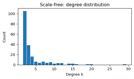
“Scale-free” in NetworkX
The BA model is the most common introduction to “scale-free” networks. NetworkX also provides other generators (some return directed multigraphs), for example:
nx.scale_free_graph(n, seed=...)nx.powerlaw_cluster_graph(n, m, p, seed=...)(adds triangle-closing for higher clustering)
For this course, nx.barabasi_albert_graph is usually the best starting point.
What’s Next?
Ready to simulate epidemics? Continue to:
References
Barabasi, Albert-Laszlo, and Reka Albert. 1999. “Emergence of Scaling in Random Networks.” Science 286 (5439): 509–12. https://doi.org/10.1126/science.286.5439.509.
Erdos, Paul, and Alfred Renyi. 1959. “On Random Graphs i.” Publicationes Mathematicae 6: 290–97.
Gilbert, Edgar N. 1959. “Random Graphs.” The Annals of Mathematical Statistics 30 (4): 1141–44. https://doi.org/10.1214/aoms/1177706098.
Newman, Mark. 2018. Networks. 2nd ed. Oxford University Press.
Watts, Duncan J., and Steven H. Strogatz. 1998. “Collective Dynamics of ’Small-World’ Networks.” Nature 393 (6684): 440–42. https://doi.org/10.1038/30918.