Kuramoto Lab: The ODE
Module 2: Synchronization and Collective Behaviour
This page covers the implementation and validation steps. You write the right-hand side of the Kuramoto model and check it in two regimes where you know the answer.
Implementation: define the ODE
Choose between the pairwise form of the Kuramoto model and the mean-field form. They are mathematically identical (The Order Parameter). The mean field approximation is often more efficient for large populations, as it avoids computing pairwise interactions.
The right-hand side only uses \(\sin\) and \(e^{i\theta}\), which are \(2\pi\)-periodic, so the dynamics do not need the phases to stay in \([0, 2\pi)\). Wrapping with np.mod(theta, 2 * np.pi) is still useful before plotting.
Exercise
Define the ODE function for the Kuramoto model and call it kuramoto_ode(). It computes the derivatives \(\dot\theta_i\) from the current phases \(\theta_i\), the natural frequencies \(\omega_i\) and the coupling strength \(K\). Follow the general template that solve_ivp() expects:
def ode(t, state, *params):
    # state represents the current values of the variables (e.g., x, y)

    # params are any additional parameters needed to compute the derivatives
    # each of them is separated by commas

    return dstate_dt  # this should be a sequence of the same length as `state`
Remember: solve_ivp() requires the time argument even if it is not used.
def kuramoto_ode(t, theta, omega, coupling_strength=1.0):
    # TODO: compute the order parameter r * exp(i * psi)

    # TODO: compute dtheta_dt with the mean-field form
    return dtheta_dt
Solution
The function below uses the mean-field form, which is cheaper than computing pairwise interactions. It computes the order parameter at each call and uses it to calculate the derivatives.
def kuramoto_ode(t, theta, omega, coupling_strength=1.0):
    # Wrapping is optional: sin and exp are 2 pi-periodic
    theta = np.mod(theta, 2 * np.pi)
    order_param = np.mean(np.exp(1j * theta))
    r = np.abs(order_param)
    phi = np.angle(order_param)
    dtheta_dt = omega + coupling_strength * r * np.sin(phi - theta)
    return dtheta_dt
Validation: two known regimes
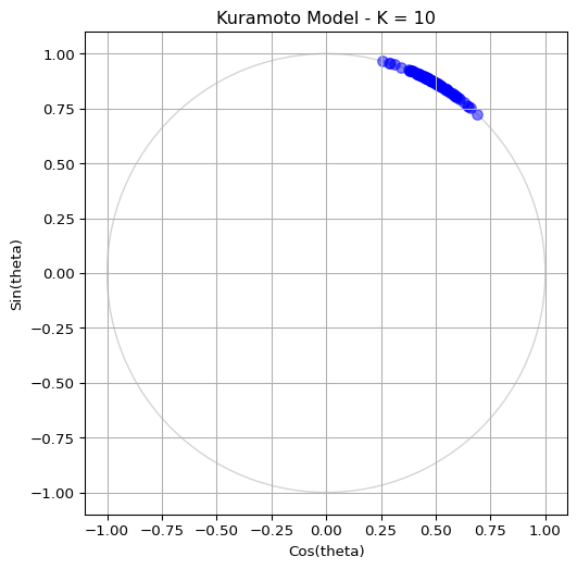
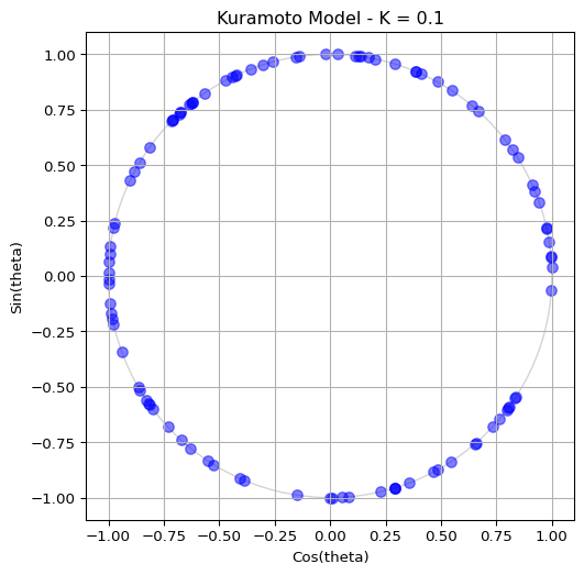
You know the answer in two regimes. For strong coupling, \(K = 10 \gg K_c\), the oscillators should cluster. For weak coupling, \(K = 0.1 \ll K_c\), they should stay spread around the circle. Figure 1 and Figure 2 show sample outputs for \(N = 100\) and \(\sigma = 1\) at \(t = 10\).
Exercise
Validate your function. Use coupling strength \(K = 10\), \(N = 100\) oscillators and \(\sigma = 1\). Integrate for \(t \in [0, 10]\) and plot the last state on the unit circle. You should see the oscillators clustering, as in Figure 1. Then reduce the coupling to \(K = 0.1\) and check that the phases stay scattered, as in Figure 2.
from scipy.integrate import solve_ivp

coupling_strength = 10.0
theta, omega = initialize_oscillators(100, sigma=1.0, seed=1)

# TODO: integrate kuramoto_ode from t = 0 to t = 10 with solve_ivp
sol =

# TODO: take the final phases and plot them on the unit circle
theta_end =
Solution
Use scipy.integrate.solve_ivp() and take the last column of sol.y.
from scipy.integrate import solve_ivp

# Parameters
coupling_strength = 10.0
num_oscillators = 100
sigma = 1.0
t_span = (0, 10)

# Initialize oscillators
theta, omega = initialize_oscillators(num_oscillators, sigma=sigma, seed=1)
# Run the simulation
sol = solve_ivp(
    kuramoto_ode,
    t_span,
    theta,
    args=(omega, coupling_strength)
    )
# The solution `sol.y` contains the phases of the oscillators at each time step.
# sol.y is a 2D array of shape (num_oscillators, num_time_points)
theta_end = sol.y[:, -1] # Get the final state of the phases
x = np.cos(theta_end)
y = np.sin(theta_end)
# Plotting code as in Initialization to visualize the final state
For the weak-coupling check, set coupling_strength = 0.1 and run the same code.
The optional page Pairwise vs Mean Field compares your function with the pairwise form.