The Central Limit Theorem
Module 3: Modelling with Randomness
Reading
- Compulsory: (newman2005power?).
- Recommended: (mantegna2000introduction?), Chapters 3 and 4.
In The Diffusion Equation the position of a walker became Gaussian after many steps. The central limit theorem (CLT) says this happens for sums of almost any independent steps, provided their variance is finite. This session is about what happens when that proviso fails.
Statement
Let \(X_1, X_2, \dots\) be independent and identically distributed with mean \(\mu\) and finite variance \(\sigma^2 > 0\). Let \(S_n = X_1 + \dots + X_n\). Then, for every real \(z\),
\[ \lim_{n \to \infty} \Pr\left( \frac{S_n - n\mu}{\sigma \sqrt{n}} \le z \right) = \Phi(z), \tag{1}\]
where \(\Phi\) is the standard normal cumulative distribution function (gnedenko1954limit?). The width of \(S_n\) grows as \(\sqrt{n}\), the same scaling as the random walk.
Assumptions
- Independence. Strongly correlated terms can change both the scaling and the limit.
- Identical distribution. Versions for non-identical terms exist (Lindeberg conditions), but no single term may dominate the sum (gnedenko1954limit?).
- Finite variance. This is the assumption that matters in this session. If \(\Pr(|X| > x)\) decays like \(x^{-\alpha}\) with \(0 < \alpha < 2\), the variance is infinite and the limit is not Gaussian (gnedenko1954limit?; mantegna2000introduction?).
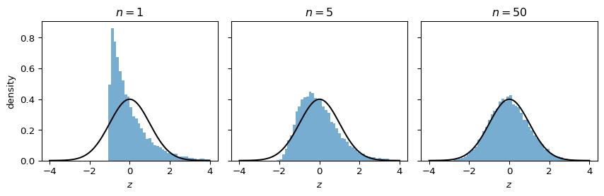
The theorem says nothing about how fast convergence happens. The tails of the distribution converge last.
A simulated check
Exponential variables are skewed, far from Gaussian. The figure standardizes sums of \(n\) of them and compares them with the standard normal density.
Exercise
Repeat the experiment with Student-t variables with 3 degrees of freedom (finite variance \(3\)) and with 1.5 degrees of freedom (infinite variance). Use rng.standard_t. For \(n = 100\), compare the fraction of standardized sums with \(|z| > 3\) to the Gaussian value \(0.0027\). For the second case, standardize by the sample standard deviation of the sums.
Solution
rng = np.random.default_rng(1)
n = 100
for df in [3.0, 1.5]:
    s = rng.standard_t(df, size=(20000, n)).sum(axis=1)
    z_s = (s - s.mean()) / s.std()
    print(f"df = {df}: fraction |z| > 3 is {np.mean(np.abs(z_s) > 3):.4f}")
df = 3.0: fraction |z| > 3 is 0.0050
df = 1.5: fraction |z| > 3 is 0.0016With 3 degrees of freedom the fraction is of the same order as the Gaussian value but still larger. The CLT holds, but the tails converge slowly. With 1.5 degrees of freedom the sample standard deviation is dominated by a few huge values; the rescaled sums pile up near zero and do not approach the normal law as \(n\) grows. The next pages explain why.