---
title: "Configuration Model"
subtitle: "Module 5: Complex Networks"
format: html
---
::: {.callout-note}
## Reading
- **Compulsory:** @newman2003structure, Section 4.2 (generalized random graphs and the configuration model), up to the clustering coefficient of Eq. (31).
- **Recommended:** @molloy1995critical for the giant component criterion, @motter2002cascade for an example of networks generated from a prescribed degree distribution.
:::
The Erdős-Rényi model fixes only the mean degree. Real networks have a degree distribution of their own, and many of the quantities of this module depend on it: the giant component after failures, the epidemic threshold and the cascade size all contain $\langle k^2 \rangle$. To study the effect of the degree distribution **alone**, we need a random graph in which the degrees are exactly those of a given network and everything else is random. This is the **configuration model**, and its sampling by *degree-preserving randomisation* is the standard null model of network science [@newman2003structure, Section 4.2].
## Definition
Given a degree sequence $(k_1, \dots, k_N)$ with an even sum, give node $i$ exactly $k_i$ "stubs" (half-edges). Pair all the stubs uniformly at random. Every graph with this degree sequence appears with the same probability, as a multigraph, that is, a graph that may contain self-loops and parallel edges [@newman2003structure, Section 4.2]. Two consequences are used throughout the module:
- Follow a random edge to the node at its other end. That node has degree $k$ with probability $k p_k / \langle k \rangle$, and so $\langle k^2 \rangle / \langle k \rangle$ neighbours on average, counting the edge we arrived by. Its *excess degree* (the number of other edges) has mean $\kappa - 1$ with $\kappa = \langle k^2 \rangle / \langle k \rangle$.
- A branching process with mean offspring $\kappa - 1$ grows if $\kappa > 2$, which is the criterion of Molloy and Reed [@molloy1995critical] used in [Robustness and Percolation](robustness-percolation.qmd).
The function below implements the definition in three lines. NetworkX has the same model as `nx.configuration_model(degree_sequence)`, which returns a `MultiGraph`.
```{python}
import matplotlib.pyplot as plt
import networkx as nx
import numpy as np
from scipy.sparse.csgraph import shortest_path

SEED = 7


def stub_matching(degrees, rng):
    """Edge list of the configuration model: shuffle the stubs and pair them."""
    stubs = np.repeat(np.arange(len(degrees)), degrees)
    rng.shuffle(stubs)
    return list(zip(stubs[::2], stubs[1::2]))


def avg_path_length(G, n_src=600, seed=0):
    """Average distance in the largest component, from at most n_src random sources."""
    H = G.subgraph(max(nx.connected_components(G), key=len))
    nodes = list(H)
    A = nx.to_scipy_sparse_array(H, nodelist=nodes, format="csr")
    # SciPy's csgraph routines require int32 CSR index buffers in this environment.
    A.indices = A.indices.astype(np.int32)
    A.indptr = A.indptr.astype(np.int32)
    n = len(nodes)
    rng = np.random.default_rng(seed)
    src = np.arange(n, dtype=np.int32) if n <= n_src else rng.choice(n, n_src, replace=False).astype(np.int32)
    return shortest_path(A, unweighted=True, indices=src).sum() / (len(src) * (n - 1))


enron = nx.Graph(nx.read_edgelist("data/ia-enron-only/ia-enron-only.edges"))
flights = nx.Graph(nx.read_graphml("data/openflights/openflights_usa.graphml.gz"))
for G in (enron, flights):
    G.remove_edges_from(nx.selfloop_edges(G))

rng = np.random.default_rng(SEED)
sequences = {
    "Poisson, <k> = 6 (N = 5000)": np.random.default_rng(1).poisson(6, 5000),
    "Barabási-Albert, m = 3 (N = 5000)": np.array([d for _, d in nx.barabasi_albert_graph(5000, 3, seed=1).degree()]),
    "Enron e-mail (N = 143)": np.array([d for _, d in enron.degree()]),
    "US flights (N = 546)": np.array([d for _, d in flights.degree()]),
}
print(f"{'degree sequence':<36}{'E':>7}{'loops':>7}{'parallel':>10}{'lost (%)':>10}")
for name, degs in sequences.items():
    degs = degs.copy()
    if degs.sum() % 2:
        degs[0] += 1
    edges = stub_matching(degs, rng)
    M = nx.MultiGraph()
    M.add_nodes_from(range(len(degs)))
    M.add_edges_from(edges)
    assert [M.degree(i) for i in range(len(degs))] == list(degs)   # degrees are exact (a loop counts twice)
    loops = nx.number_of_selfloops(M)
    S = nx.Graph(M)
    S.remove_edges_from(nx.selfloop_edges(S))
    parallel = M.number_of_edges() - loops - S.number_of_edges()   # edges merged into an existing one
    print(f"{name:<36}{len(edges):>7}{loops:>7}{parallel:>10}{100 * (loops + parallel) / len(edges):>10.1f}")
```
The degrees are exact. Every degree sequence produces some self-loops and parallel edges, and their share grows with the heterogeneity of the sequence: two hubs $i$ and $j$ are expected to be joined by $k_i k_j / 2E$ edges, which is larger than one when both degrees are large. Removing the loops and merging parallel edges ("erasing") gives a simple graph, but it no longer has the original degrees. For a sparse and homogeneous sequence the loss is small; for the flights sequence it is a sizeable fraction of the edges.
## Degree-preserving randomisation
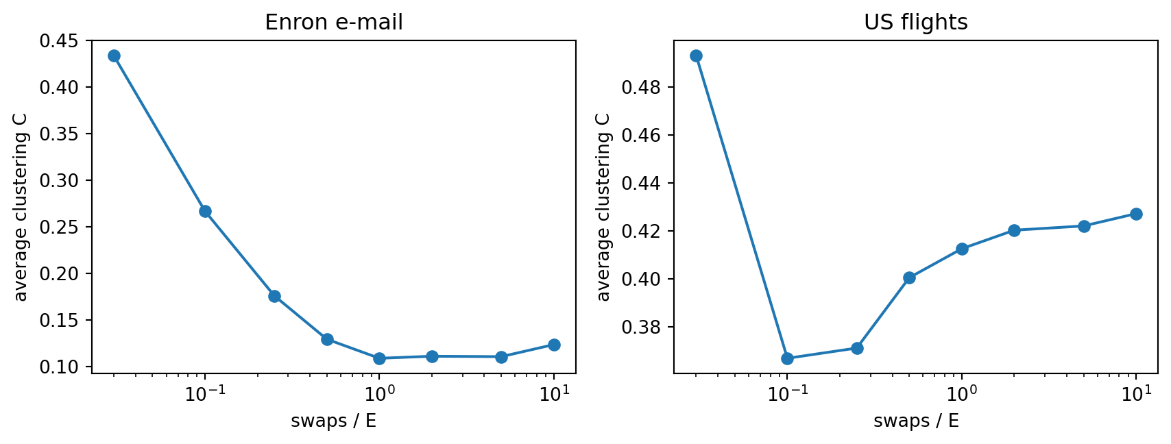
To sample **simple** graphs with exactly the degrees of an observed network, start from the network and repeat a **double-edge swap**: pick two edges $(u,v)$ and $(x,y)$ and replace them by $(u,x)$ and $(v,y)$, unless one of these edges already exists. Each swap keeps every degree, so after many swaps the graph is a sample of the simple-graph version of the configuration model. In NetworkX the function is `nx.double_edge_swap(G, nswap, max_tries)`. How many swaps are enough? @fig-swap-convergence follows the clustering of the two data networks as a function of the number of swaps in units of $E$.
```{python}
#| label: fig-swap-convergence
#| fig-cap: "Average clustering coefficient of the Enron and US flights networks during degree-preserving randomisation, against the number of double-edge swaps in units of the number of edges E. Lines are averages over 3 runs; the starting values (plotted at 0.03) are the clustering of the original networks. The Enron curve flattens after about E swaps. The flights curve drops in the first 0.1E swaps, then recovers slowly and is flat from about 2E swaps on."
fig, axes = plt.subplots(1, 2, figsize=(9, 3.5))
swaps_E = np.array([0, 0.1, 0.25, 0.5, 1, 2, 5, 10])
for ax, (name, G) in zip(axes, [("Enron e-mail", enron), ("US flights", flights)]):
    E = G.number_of_edges()
    curves = []
    for r in range(3):
        H = G.copy()
        values, done = [], 0
        for s in swaps_E:
            todo = int(s * E) - done
            if todo > 0:
                nx.double_edge_swap(H, nswap=todo, max_tries=100 * E, seed=SEED + r + done)
                done += todo
            values.append(nx.average_clustering(H))
        assert sorted(d for _, d in H.degree()) == sorted(d for _, d in G.degree())
        curves.append(values)
    ax.semilogx(np.maximum(swaps_E, 0.03), np.mean(curves, axis=0), "o-")
    ax.set_xlabel("swaps / E")
    ax.set_ylabel("average clustering C")
    ax.set_title(name)
plt.tight_layout()
plt.show()
print("the assertion inside the loop checks that the degree sequence never changes")
```
The Enron clustering levels off after about $E$ swaps. The flights clustering is not monotone: the first swaps remove the triangles, and then it recovers slowly as the hubs rearrange, to a plateau from about $2E$ swaps on. We use $10E$ swaps below. (The plot checks only one quantity; other properties may need more swaps.)
## How much of the clustering is explained by the degrees?
A standard question compares the clustering of a real network with that of a random graph. The answer depends on which random graph. The table compares each data network with two nulls: the Erdős-Rényi graph $G(N, E)$, which keeps only the number of nodes and edges, and the degree-preserving randomisation, which also keeps every degree. It shows the average of the local clustering coefficients, the *transitivity* (three times the number of triangles divided by the number of connected triples [@newman2003structure, Eq. (3)], `nx.transitivity`), the average path length and the degree assortativity coefficient $r$ (the correlation between the degrees at the two ends of an edge).
```{python}
#| label: tbl-null-models
#| tbl-cap: "Real networks against two null models, averaged over 5 realisations of each null. C is the average local clustering, T the transitivity, L the average path length in the largest component and r the degree assortativity coefficient. Enron: 143 nodes and 623 edges; US flights: 546 nodes and 2781 edges."
def profile(G):
    return dict(C=nx.average_clustering(G), T=nx.transitivity(G), L=avg_path_length(G),
                r=nx.degree_assortativity_coefficient(G))


print(f"{'network / null':<28}{'C':>8}{'T':>8}{'L':>7}{'r':>8}")
for name, G in [("Enron", enron), ("US flights", flights)]:
    N, E = G.number_of_nodes(), G.number_of_edges()
    er = [profile(nx.gnm_random_graph(N, E, seed=SEED + s)) for s in range(5)]
    sw = []
    for s in range(5):
        H = G.copy()
        nx.double_edge_swap(H, nswap=10 * E, max_tries=100 * E, seed=SEED + s)
        sw.append(profile(H))
    for label, rows in [("real", [profile(G)]), ("G(N, E)", er), ("degree-preserving", sw)]:
        m = {key: np.mean([row[key] for row in rows]) for key in rows[0]}
        print(f"{name + ' ' + label:<28}{m['C']:>8.3f}{m['T']:>8.3f}{m['L']:>7.2f}{m['r']:>8.2f}")
```
Two lessons follow.
- **The conclusion depends on the null.** The Enron network has $C = 0.43$ against $0.06$ for $G(N,E)$ and $0.11$ for the degree-preserving null: the clustering is high even after the degrees are taken into account, which is consistent with a triadic-closure mechanism. The flights network has $C = 0.49$ against $0.02$ for $G(N,E)$, but $0.43$ for the degree-preserving null: most of the local clustering comes from the degree sequence. The airports of degree 2 or 3 have a mean local clustering of 0.79 in the data; when such a small node is attached to two large hubs, the hubs are very likely to be linked to each other, even in a random graph with the same degrees. The transitivity tells a more cautious story, with a smaller excess over the null.
- **Simple graphs with hubs are disassortative.** The degree-preserving null of the flights network has $r \approx -0.4$, close to the real value, because hubs cannot have many parallel edges and so are joined mostly to small nodes. The assortativity of the flights network is largely explained by the degree sequence as well.
## A formula for the clustering of the configuration model
For the configuration model, the transitivity is
$$
T = \frac{1}{N}\,\frac{\big(\langle k^2 \rangle - \langle k \rangle\big)^2}{\langle k \rangle^3},
$$ {#eq-cm-clustering}
the value $\langle k \rangle / N$ of the Poisson random graph times a factor that grows with the width of the degree distribution [@newman2003structure, Eq. (31)]. It goes to zero as $1/N$ for a fixed distribution, unless $\langle k^2 \rangle$ grows with $N$. The next chunk tests the formula on random power-law sequences ($p_k \propto k^{-\gamma}$, minimum degree $k_{\min}$, maximum degree $\sqrt{3N}$) and on the two data networks.
```{python}
def power_law_sequence(N, gamma, kmin, kmax, rng):
    ks = np.arange(kmin, kmax + 1)
    p = ks ** (-gamma)
    s = rng.choice(ks, N, p=p / p.sum())
    if s.sum() % 2:
        s[0] += 1
    return s


def eq_cm(degs):
    k = np.asarray(degs, dtype=float)
    return ((k**2).mean() - k.mean()) ** 2 / (len(k) * k.mean() ** 3)


rng = np.random.default_rng(SEED)
print(f"{'sequence':<26}{'N':>7}{'k_max':>7}{'formula':>9}{'measured':>10}")
for gamma, kmin in [(3.0, 3), (2.5, 2)]:
    for N in (2000, 8000, 32000):
        s = power_law_sequence(N, gamma, kmin, int(np.sqrt(3 * N)), rng)
        T = []
        for r in range(3):
            G = nx.Graph(nx.configuration_model(list(s), seed=SEED + r))
            G.remove_edges_from(nx.selfloop_edges(G))
            T.append(nx.transitivity(G))
        print(f"{f'gamma = {gamma}, kmin = {kmin}':<26}{N:>7}{s.max():>7}{eq_cm(s):>9.4f}{np.mean(T):>10.4f}")
for name, G in [("Enron e-mail", enron), ("US flights", flights)]:
    degs = [d for _, d in G.degree()]
    H = G.copy()
    nx.double_edge_swap(H, nswap=10 * G.number_of_edges(), max_tries=10**7, seed=SEED)
    print(f"{name:<26}{len(G):>7}{max(degs):>7}{eq_cm(degs):>9.4f}{nx.transitivity(H):>10.4f}"
          f"   (sqrt(2E) = {np.sqrt(2 * G.number_of_edges()):.0f})")
```
For the synthetic sequences the formula is accurate to within about 20%. For the Enron network it agrees closely with the degree-preserving null. For the flights network it overestimates by a factor of more than two. In that network the largest degree (153) is twice $\sqrt{2E} \approx 75$: hubs of that size would need parallel edges, which a simple graph does not allow, so the simple null has fewer triangles around them than the multigraph formula assumes. The formula is a result for $N \to \infty$ with bounded $k_{\max}/\sqrt{N}$; use the numerical null whenever the largest degrees are comparable to $\sqrt{2E}$.
## Does clustering matter for spreading?
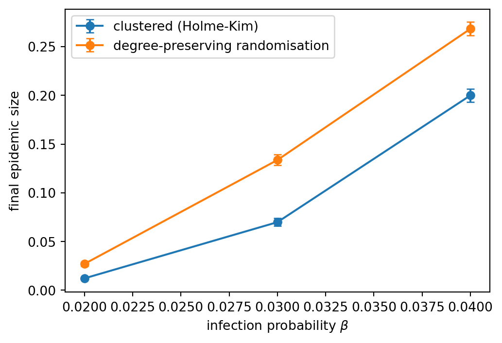
The heterogeneous mean-field threshold of [Epidemic Threshold](epidemic-threshold.qmd) uses only $p_k$. The configuration model lets us test the effect of everything else. Take a clustered scale-free graph from [Triadic Closure](triadic-closure.qmd) ($N = 3000$, $m = 3$, $p_t = 0.9$), randomise it with $10E$ double-edge swaps, and run the discrete-time SIR model of [SIR on Networks](sir-network.qmd) on both. The swapped graph has the same degrees and almost no triangles; it also loses any degree correlations of the original, so the comparison measures the effect of all the structure beyond the degrees.
```{python}
#| label: fig-sir-clustering
#| fig-cap: "Mean final epidemic size (fraction of nodes ever infected) of the discrete-time SIR model with recovery probability 0.2 and 5 initial infected nodes, on a clustered Holme-Kim graph (N = 3000, m = 3, p_t = 0.9, C = 0.52) and on its degree-preserving randomisation (C = 0.01). 400 runs per point; error bars are one standard error."
from amlab.networks_spreading import run_sir_fast

G_hk = nx.powerlaw_cluster_graph(3000, 3, 0.9, seed=2)
G_sw = G_hk.copy()
nx.double_edge_swap(G_sw, nswap=10 * G_sw.number_of_edges(), max_tries=10**7, seed=2)
print(f"C: clustered = {nx.average_clustering(G_hk):.2f}, randomised = {nx.average_clustering(G_sw):.3f}")

rng = np.random.default_rng(5)
betas = [0.02, 0.03, 0.04]
fig, ax = plt.subplots(figsize=(5.5, 3.8))
for G, label in [(G_hk, "clustered (Holme-Kim)"), (G_sw, "degree-preserving randomisation")]:
    means, errs = [], []
    for beta in betas:
        sizes = np.array([run_sir_fast(G, beta, 0.2, initial_infected=5, rng=rng) for _ in range(400)])
        means.append(sizes.mean())
        errs.append(sizes.std() / np.sqrt(len(sizes)))
    ax.errorbar(betas, means, yerr=errs, fmt="o-", capsize=3, label=label)
    print(label, np.round(means, 3))
ax.set_xlabel(r"infection probability $\beta$")
ax.set_ylabel("final epidemic size")
ax.legend()
plt.tight_layout()
plt.show()
```
At $\beta = 0.02$ and $0.03$, close to the threshold, the clustered network has a final size that is 0.4 to 0.5 times that of its degree-preserving randomisation; at $\beta = 0.04$ the ratio is 0.75. Clustering wastes infection attempts: when two neighbours of an infected node are themselves neighbours, one of them may already have been infected through the other. The effect shrinks as the infection probability grows. The mean-field formula for $\lambda_c$ has no term for it [@pastor2015epidemic].
::: {.callout-note}
## Exercise
(a) Using the table of this page, compute for each data network the ratio between the real transitivity and the transitivity of the degree-preserving null. (b) A student states that "the flights network is clustered like a social network, so triadic closure must be at work". Evaluate the statement with the two nulls.
:::
::: {.callout-tip collapse="true"}
## Solution
(a) Enron: $0.359/0.114 \approx 3.1$. Flights: $0.313/0.229 \approx 1.4$. (b) Against $G(N,E)$ the average clustering of the flights network is 27 times larger, which looks like strong evidence. Against the degree-preserving null the local clustering is only 1.15 times larger ($0.49$ against $0.43$) and the transitivity 1.4 times larger. Most of the apparent clustering is a consequence of the hubs, so the evidence for a triadic-closure mechanism is weak; the Enron network, with a factor of 3 in transitivity, is much stronger evidence. The right null for a statement about a mechanism is the one that keeps everything the mechanism is not supposed to explain.
:::
::: {.callout-note}
## Exercise
Use `nx.configuration_model` on the degree sequence of the flights network and convert the result to a simple graph with `nx.Graph(M)` and `M.remove_edges_from(nx.selfloop_edges(M))`. How many edges are lost? How do the clustering and the largest degree of the simple graph compare with the original?
:::
::: {.callout-tip collapse="true"}
## Solution
```python
degs = [d for _, d in flights.degree()]
M = nx.configuration_model(degs, seed=1)
S = nx.Graph(M)
S.remove_edges_from(nx.selfloop_edges(S))
print(flights.number_of_edges(), S.number_of_edges(), max(d for _, d in S.degree()))
```
With `seed=1` the simple graph keeps 2293 of the 2781 edges (82%), because self-loops and merged parallel edges are lost, its largest degree is 95 instead of 153, and its average clustering is 0.19 against 0.49 for the original. This is why the degree-preserving swap is the better null for heterogeneous sequences.
:::
## What's Next?
The configuration model is the setting in which the Molloy-Reed criterion and the heterogeneous mean-field threshold hold exactly. [SIR and Percolation](sir-percolation.qmd) uses it to connect epidemic outbreaks to the robustness results of [Robustness and Percolation](robustness-percolation.qmd).