Reaction-Diffusion Equations
Module 4: Space and Pattern Formation
Reading
- Compulsory: (murray2002mathematical?), Chapter 11 (Reaction Diffusion, Chemotaxis, and Nonlocal Mechanisms).
- Recommended: (britton2003essential?), Chapter 5 (Biological Motion) and Chapter 7 (Pattern Formation).
In Module 3 you derived the diffusion equation \(\partial_t c = D\,\partial_{xx} c\) as the continuum limit of a random walk (From random walks to diffusion). A reaction-diffusion equation adds local production and decay to that transport term (murray2002mathematical?).
The General Form
For \(m\) species with concentrations \(w = (w_1, \dots, w_m)\) on a domain \(\Omega\),
\[ \partial_t w = D\,\Delta w + R(w), \qquad D = \operatorname{diag}(D_1, \dots, D_m). \tag{1}\]
- \(\Delta\) is the Laplacian, \(\partial_{xx}\) in 1D and \(\partial_{xx} + \partial_{yy}\) in 2D.
- \(D_i > 0\) is the diffusion coefficient of species \(i\).
- \(R(w)\) collects the reaction kinetics. With \(D = 0\) you recover an ODE system at every point, as in Module 1.
The model is incomplete without an initial condition \(w(x, 0)\) and boundary conditions on \(\partial\Omega\). You will meet Neumann (zero flux), Dirichlet (fixed value), and periodic conditions on the page Laplacian Eigenmodes.
The Scaling Used in This Module
For two species \(u\) and \(v\) we use the nondimensional form of (murray2003mathematical?):
\[ \begin{aligned} \partial_t u &= \Delta u + \gamma f(u, v), \\ \partial_t v &= d\,\Delta v + \gamma g(u, v). \end{aligned} \tag{2}\]
Here \(d = D_v / D_u\) is the ratio of diffusion coefficients and \(\gamma\) measures the strength of the reactions relative to diffusion. In Murray’s scaling \(\gamma\) is proportional to the square of the domain length, so increasing \(\gamma\) at fixed domain is equivalent to enlarging the domain (murray2003mathematical?). The Gierer-Meinhardt code in amlab.pdes_1d and amlab.pdes_2d uses exactly these symbols.
Examples
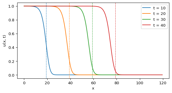
- Fisher-KPP equation. One species, logistic growth plus diffusion: \(\partial_t u = D\,\partial_{xx} u + r u(1-u)\). It was proposed for the spread of an advantageous gene (fisher1937wave?). It has travelling fronts with minimal speed \(c = 2\sqrt{rD}\) (murray2002mathematical?).
- Gierer-Meinhardt model. An activator \(u\) and an inhibitor \(v\) with \(f = a - bu + u^2/v\) and \(g = u^2 - v\) (Gierer and Meinhardt 1972). It forms stationary patterns and is the main example of this module.
- Gray-Scott model. An autocatalytic reaction with feed and removal (Gray and Scott 1984). Its 2D simulations produce spots, stripes and self-replicating spots (Pearson 1993).
- Chemical experiments. Stationary Turing patterns were first observed experimentally in the CIMA reaction (castets1990experimental?).
A First Simulation
Figure 1 shows a Fisher-KPP front with \(D = r = 1\). The dashed lines move at the predicted speed \(c = 2\).
For an initial condition with compact support the front speed tends to the minimal speed \(c = 2\sqrt{rD}\) as \(t \to \infty\) (murray2002mathematical?).
Exercise
Set \(D = 0\) in Equation 1. What happens to a spatial profile \(u(x, 0)\) under Fisher-KPP kinetics, and why can no front move?
Solution
Each point solves the logistic ODE \(\dot u = r u (1-u)\) independently. Points with \(u(x,0) > 0\) grow to \(1\) and points with \(u(x,0) = 0\) stay at \(0\). Without diffusion no point can influence its neighbours, so the region with \(u = 0\) never becomes invaded.
References
Gierer, Alfred, and Hans Meinhardt. 1972. “A Theory of Biological Pattern Formation.” Kybernetik 12 (1): 30–39. https://doi.org/10.1007/BF00289234.
Gray, Peter, and Stephen K. Scott. 1984. “Autocatalytic Reactions in the Isothermal, Continuous Stirred Tank Reactor: Isolas and Other Forms of Multistability.” Chemical Engineering Science 39 (6): 1087–97. https://doi.org/10.1016/0009-2509(84)87017-7.
Pearson, John E. 1993. “Complex Patterns in a Simple System.” Science 261 (5118): 189–92. https://doi.org/10.1126/science.261.5118.189.