---
title: "Dictyostelium: Amoebae That Pass a Signal"
subtitle: "Module 7: Combining Ideas"
format: html
---
::: {.callout-tip}
## Optional extension
This page combines two ideas from earlier modules, **agents that move and interact locally** (Module 2, see the [Vicsek model](../collective-behaviour/vicsek-model.qmd) and the [Couzin model](../collective-behaviour/couzin-model.qmd)) and **an excitable field that spreads, fires and recovers** (reaction-diffusion and fast-slow dynamics, Modules 1 and 4; see the [FitzHugh-Nagumo model](../low-dimensional-dynamics/fitzhugh-nagumo.qmd) for excitable kinetics, the [Gray-Scott model](../pattern-formation/gray-scott.qmd) for a reaction-diffusion field, and the [fast-slow budworm model](../low-dimensional-dynamics/budworm-forest-fast-slow.qmd) for the idea of a slow variable that switches a fast one off). The question is: **can a crowd of cells gather at one place without any leader, only by passing a signal on and walking toward it?**
:::
The social amoeba *Dictyostelium discoideum* lives as single cells in the soil. When the food runs out, the cells start to secrete the small molecule cyclic AMP (cAMP) and to detect it. Secretion is a **relay**: a cell that senses cAMP above a threshold secretes cAMP itself, and then it needs time to recover before it can respond again. The cAMP therefore travels through the population as a **wave**, and the cells walk toward the source of each wave. After many waves thousands of cells have gathered in a few clusters, and each cluster becomes a multicellular body. The one-sentence story of the model is:
> **Amoebae pass a signal along and walk toward it, so they gather without a leader.**
Time-lapse measurements of starving populations show spiral waves of cAMP with periods between 3.5 and 5.5 minutes, and cells that move toward the wave source at the wave fronts [@ford2023spirals]. Mathematical models of the relay go back to a receptor-desensitisation model of the cAMP signalling [@martiel1987model], and a cell-based excitable model reproduces circular waves and spirals in aggregation territories [@palsson1996cell]. A book chapter by Siegert and Weijer [@siegertweijer] reviews the role of periodic signals in the morphogenesis of *Dictyostelium*; it is a pointer for further reading.
We use the simplest model that has the two ingredients and their coupling, and we say clearly what it leaves out.
::: {.callout-note}
## What is and is not claimed
This is a **teaching model**. Space and time are in model units (grid spacings and the time scale $1/k$ of the reaction), and no parameter is fitted to data. I do not state a wave period in minutes for the model, because I cannot map its time units to measurements honestly. What the model is meant to show is a mechanism: an excitable medium plus a **rising-front rule** for the cells is enough to turn random firing into waves and waves into clusters. It does **not** reproduce the sustained spirals seen in experiments (see the reality check below).
:::
## The model
Cells live on a square dish of $100 \times 100$ grid sites with grid spacing $\Delta x = 1$ and no-flux walls. The field lives on the same grid.
| Ingredient | Rule |
|---|---|
| **Field $u$** | Extracellular cAMP. It diffuses (coefficient $D$), is secreted in a relay with a threshold $\theta$, and is degraded at a small rate $\mu$. |
| **Field $v$** | A slow recovery variable: the refractory state of the relaying cells. It rises while $u$ is high and switches the relay off. |
| **Relay capacity $g(\mathbf x)$** | The local cell density, smoothed over a few sites and divided by $\rho_c$, clipped to $[0, 1]$. Where there are no cells, the medium cannot relay and cAMP only decays. |
| **Spontaneous firing** | Every cell fires at random with a small rate. A firing adds a Gaussian bump of cAMP of radius 3.5 sites. The bump becomes a wave only if the medium has recovered and has enough cells. |
| **Cells** | Points with a heading. They walk slowly and at random. While the cAMP at the cell is **rising**, the cell turns toward the gradient $\nabla u$ and walks with the chemotactic speed $v_\text{chem}$ for a time $t_\text{chem}$. |
### The field: an excitable medium
The kinetics are of Barkley and FitzHugh-Nagumo type: a cubic activator $u$ and a slow linear inhibitor $v$.
$$
\frac{\partial u}{\partial t} = D\,\nabla^2 u + k\,g(\mathbf x)\,u\,(1-u)\,(u - \theta - \gamma v) - \mu\,u ,
$$ {#eq-field}
$$
\frac{\partial v}{\partial t} = \varepsilon\,(u - v) .
$$ {#eq-recovery}
The cubic has the roots $u = 0$ (rest), $u = 1$ (excited) and $u = \theta + \gamma v$ (the threshold). A bump of $u$ above the threshold grows to the excited state. Then $v$ rises at the slow rate $\varepsilon$, the threshold $\theta + \gamma v$ climbs, the excited state disappears and the medium falls back to rest. While $v$ is still high, the threshold is too high to excite the medium again: this is the **refractory period**, and it is why waves do not run backward. The default values are $D = 1$, $k = 1$, $\theta = 0.15$, $\gamma = 1.2$, $\varepsilon = 0.025$ and $\mu = 0.005$.
The relay capacity of @eq-field is a coarse-grained version of "a cell that senses cAMP above threshold secretes cAMP":
$$
g(\mathbf x) = \min\!\left(1,\ \frac{\bar\rho(\mathbf x)}{\rho_c}\right),
$$ {#eq-gain}
where $\bar\rho$ is the cell density (cells per site) smoothed with a $[1, 2, 1]/4$ kernel applied twice in each direction. With the default $\rho_c = 0.06$, a medium with more than 0.06 cells per site relays at full strength, and a dish that is emptied of cells can no longer carry a wave. Hence **the waves feel the cells**, and the cells feel the waves.
### How fast does a front travel?
Set $v = 0$, $\mu = 0$ and $g = 1$ in @eq-field. What is left is the Nagumo equation, whose travelling front has an exact speed (Exercise 1 derives it):
$$
c = \sqrt{\frac{D k}{2}}\,\bigl(1 - 2\theta\bigr) .
$$ {#eq-speed}
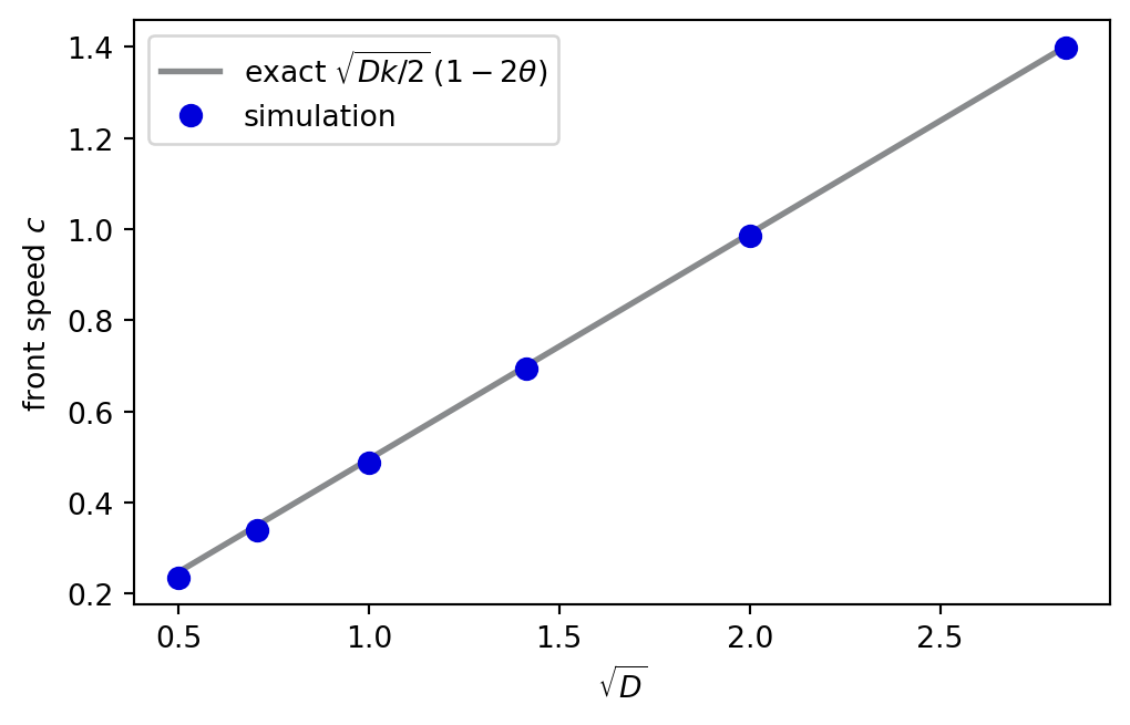
The speed grows with the square root of the product of the diffusion coefficient and the reaction rate. A length $\sqrt{D/k}$ (the width of the front) and a time $1/k$ (the time it takes to switch) can be combined into a speed in only one way. A cell that senses cAMP at the front sees it rise within a few time units, which is what the cells use. The next chunk measures the front speed in the simulation and compares it with @eq-speed.
```{python}
#| label: fig-front-speed
#| fig-cap: "Front speed of the pure excitable field (no recovery, no degradation, no cells) for several diffusion coefficients, against the exact Nagumo speed. Both axes are linear; the speed rises like the square root of D."
#| fig-alt: "A plot of front speed against the square root of D. Six measured points lie on a straight line that rises from about 0.25 at 0.5 to about 1.4 at 2.8, and an exact line through them is almost indistinguishable."
import numpy as np
import matplotlib.pyplot as plt
from amlab.collective_motion.dicty import front_speed, nagumo_speed

D = np.array([0.25, 0.5, 1.0, 2.0, 4.0, 8.0])
measured = np.array([front_speed(d) for d in D])
exact = np.array([nagumo_speed(d, 1.0, 0.15) for d in D])

fig, ax = plt.subplots(figsize=(5.2, 3.3), constrained_layout=True)
ax.plot(np.sqrt(D), exact, "-", lw=2, color="#888A8C", label="exact $\\sqrt{Dk/2}\\,(1-2\\theta)$")
ax.plot(np.sqrt(D), measured, "o", ms=7, color="#0000DB", label="simulation")
ax.set_xlabel("$\\sqrt{D}$")
ax.set_ylabel("front speed $c$")
ax.legend()
plt.show()
for d, m_, e in zip(D, measured, exact):
    print(f"D = {d:4.2f}: measured {m_:.3f}, exact {e:.3f}, ratio {m_ / e:.3f}")
```
### The cells: a ratchet that works only on rising fronts
A cell cannot sense a gradient across its own body in the model, but it can sense how the cAMP at its position **changes in time**. Let $\dot u_i = (u(\mathbf x_i, t) - u(\mathbf x_i, t - \Delta t))/\Delta t$. The cell $i$ with heading $h_i$ follows
$$
\begin{aligned}
&\text{if } \dot u_i > r:\quad h_i \leftarrow \operatorname{atan2}\!\left(\partial_y u,\ \partial_x u\right),\quad \tau_i \leftarrow t_\text{chem}, \\
&\text{speed} = v_\text{chem} \ \text{ while } \tau_i > 0, \ \text{ otherwise } v_0 ; \qquad \tau_i \leftarrow \tau_i - \Delta t, \\
&dh_i = \sqrt{2 d_\text{rot}\,\Delta t}\ \xi_i , \quad \xi_i \sim \mathcal N(0, 1) .
\end{aligned}
$$ {#eq-cells}
While the cAMP rises at the cell, the front of a wave is passing, and $\nabla u$ points **toward the source**, because the cAMP is higher behind the front. After the wave has passed, the cAMP falls and the gradient points away from the source; the cell ignores it. Every wave therefore moves each cell a short step toward its source. This **ratchet** is the same idea as the cell behaviour reported at wave fronts [@ford2023spirals], in a very reduced form.
| Parameter | Value | | Parameter | Value |
|---|---|---|---|---|
| diffusion $D$, reaction rate $k$ | 1, 1 | | threshold $\theta$ (the **excitability dial**) | 0.15 |
| recovery rate $\varepsilon$, inhibition $\gamma$ | 0.025, 1.2 | | degradation $\mu$ | 0.005 |
| relay density $\rho_c$ | 0.06 cells per site | | cell density (a **dial**) | 0.30 cells per site (3000 cells) |
| random speed $v_0$, rotational diffusion $d_\text{rot}$ | 0.02, 0.05 | | chemotactic speed $v_\text{chem}$ (a **dial**) | 0.30 |
| directed time $t_\text{chem}$, rise threshold $r$ | 6, 0.04 | | firing rate per cell | $4 \times 10^{-5}$ per time unit |
| time step $\Delta t$ | 0.2 | | grid | $100 \times 100$, $\Delta x = 1$ |
The scheme is explicit Euler in time and the five-point stencil in space. It is stable only if $\Delta t \le \Delta x^2/(4D)$ (Exercise 2). With $D = 1$ the limit is 0.25, and we use 0.2. The `self_test()` of the code checks this limit.
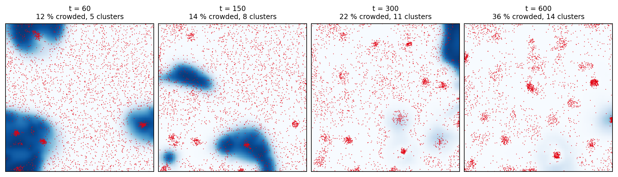
One run looks like this. At the start the cells are spread evenly and the field is at rest. Random firings start the first waves, and the cells that feel a front walk toward its centre. The next chunk shows four snapshots of the same run.
```{python}
#| label: fig-scene
#| fig-cap: "One run with the default parameters. Colour is the cAMP field u (dark blue: a wave), dots are cells. Large waves pass early; at later times small tight clusters appear, each at the centre of its own territory, and a part of the cells is still spread out."
#| fig-alt: "Four square maps of the dish at times 60, 150, 300 and 600. At time 60 three dark-blue waves cover parts of the dish and the cells are spread evenly, with 12 percent in crowded blocks. At 150 and 300 the waves are smaller and small red clusters of cells appear on a pale background, 8 and 11 clusters. At 600 there are 14 tight clusters that hold 36 percent of the cells; the others are still spread over the dish."
import numpy as np
import matplotlib.pyplot as plt
from amlab.collective_motion.dicty import DictyParams, DictySimulation

sim = DictySimulation(DictyParams(), seed=3)
fig, axs = plt.subplots(1, 4, figsize=(11, 3.1), constrained_layout=True)
for ax, t in zip(axs, (60, 150, 300, 600)):
    sim.run(t - sim.time)
    ax.pcolormesh(sim.u.T, vmin=0, vmax=1, cmap="Blues")
    ax.scatter(sim.x, sim.y, s=0.8, color="#E2000F", linewidths=0)
    a = sim.aggregation()
    ax.set_title(f"t = {t}\n{100 * a['share']:.0f} % crowded, {a['clusters']:.0f} clusters", fontsize=9)
    ax.set_xticks([]); ax.set_yticks([]); ax.set_aspect("equal")
plt.show()
```
## Explore the dish
The figure is the same model, ported to JavaScript. The colour is the cAMP field: dark blue is rest, white is a wave front. A **small round dot** is a cell at rest or moving at random; a **larger triangle with a white edge** is a cell that has just sensed a rising front and is walking toward it. The text in the corner and the readout below the figure give the share of cells in crowded blocks, the number of crowded clusters and the area that is excited, so no information depends on colour alone. The plot shows the share and the excited area over the last 600 time units. Click the dish and press **Space** to pause or **N** for a new run.
::: {.viz data-viz="dicty"}
1. Watch the first 100 time units without touching anything. Where do the first waves start, and what happens to the cells that a front passes? Why do the waves stop at the edges of the empty regions?
2. Set the **chemotactic speed** to 0. The waves still run, but the share of cells in crowded blocks stays near zero. Which part of the story is missing?
3. Raise the **threshold** $\theta$ from 0.15 to 0.35. The medium becomes less excitable. How do the fronts change, and how do the clusters change after 500 time units? (Use @eq-speed to predict the change in speed.)
4. Lower the **cell density** to 0.1 and release the slider. Aggregation still happens, but more slowly and with less of the cell population in clusters. Then try 0.6. Does a denser population give more or fewer clusters?
5. Press **New run** several times with the default dials. Does the number of clusters vary from run to run? Which dial changes it most?
6. Raise the **Speed** to 8 to watch a whole aggregation in about a minute. The simulation is the same; only the number of steps per frame changes.
:::
## Run it on your computer
From the repository root:
```bash
# the animation with sliders (IE dark theme)
python amlab/collective_motion/dicty_animation.py

# options: light theme, sparser cells, a control without chemotaxis
python amlab/collective_motion/dicty_animation.py --theme light --density 0.15
python amlab/collective_motion/dicty_animation.py --no-chemotaxis

# save a GIF or an MP4 (needs ffmpeg), or one PNG picture, instead of opening a window
python amlab/collective_motion/dicty_animation.py --save dicty.gif --frames 400
python amlab/collective_motion/dicty_animation.py --save dicty.png --frames 900

# self-test and a short comparison with and without chemotaxis, without graphics
python amlab/collective_motion/dicty.py
```
In the window, the sliders change the threshold and the chemotactic speed live, and the cell density restarts the run. **New run** (or **N**) starts again and **Space** pauses. The animation redraws only the moving parts (blitting); use `--speed 2` on a slow computer.
## How the code works
The model is in `amlab/collective_motion/dicty.py`. The Laplacian of @eq-field uses differences between neighbours. Because a difference is only taken where two sites exist, the walls are no-flux without any extra rule:
```python
d = a[1:] - a[:-1]                  # flux between neighbours in x
lap[:-1] += d; lap[1:] -= d
d = a[:, 1:] - a[:, :-1]            # and in y
lap[:, :-1] += d; lap[:, 1:] -= d
```
The reaction and the update are one line each (@eq-field and @eq-recovery):
```python
react = k * gain * u * (1 - u) * (u - theta - gamma * v) - mu * u
u, v = u + dt * (D * lap + react), v + dt * eps * (u - v)
```
and the cells of @eq-cells read the field at their own site:
```python
du = (u_here - u_prev) / dt                 # rate of change at the cell
rising = du > rise
h[rising] = np.arctan2(gy[rising], gx[rising])   # turn toward the gradient
timer[rising] = t_chem                       # walk for a while
speed = np.where(timer > 0, v_chem, v0)
```
`self_test()` checks that the same seed gives the same run, that the explicit scheme is stable at $\Delta t\,D/\Delta x^2 = 0.2$ and blows up at 0.4, that $u$ and $v$ stay in $[0, 1]$ with no NaN over a long run, that diffusion alone conserves $u$, that the measured front speed is within 8% of @eq-speed for four values of $D$ and doubles when $D$ is multiplied by 4, that a bump in the refractory wake starts no wave, and that cells move toward a wave source with chemotaxis on and do not with it off.
To run your own experiment:
```python
from dataclasses import replace
from amlab.collective_motion.dicty import DictyParams, sweep

res = sweep("theta", [0.1, 0.2, 0.3], base=DictyParams(), n_seeds=20, t_max=1500.0)
print(res["values"], res["share"], res["clusters"])
```
`sweep` runs `n_seeds` independent runs for every value and returns the means of the final aggregated share and of the final number of clusters. The next chunk is a small version of the experiment below (3 seeds and a short run), only to show the helper at work.
```{python}
#| label: tbl-quick
from dataclasses import replace
import numpy as np
from amlab.collective_motion.dicty import DictyParams, run

base = DictyParams()
for label, par in [("chemotaxis off", replace(base, chemotaxis=False)), ("chemotaxis on", base)]:
    res = [run(par, seed, t_max=400.0) for seed in range(3)]
    print(f"{label:15s} share of cells in crowded blocks {np.mean([r['share'] for r in res]):.2f}, "
          f"clusters {np.mean([r['clusters'] for r in res]):4.1f}, spontaneous firings {np.mean([r['fired'] for r in res]):5.1f}")
```
## Experiment: how many cells gather, and how many clusters form?
`run_dicty_experiments.py run --seeds 20` reproduces the figure below. A run lasts 1500 time units. The **aggregated share** is the fraction of cells that sit in *crowded blocks*: the dish is cut into $5 \times 5$ blocks, and a block is crowded if it holds more than four times the mean number of cells per block. A **cluster** is a group of crowded blocks that touch along an edge. Both numbers are measured at $t = 1500$. The **time to aggregate** is the first time (sampled every 20 time units) at which the share reaches 50%; if it never does, it is recorded as 1500, so the mean is cut off. Every single run is saved in `data/dicty_runs.csv`. Each setting has **20 independent runs** (seeds 0 to 19: different starting positions of the cells and different spontaneous firings). Error bars are 95% confidence intervals for the mean, $1.96\,s/\sqrt{20}$.
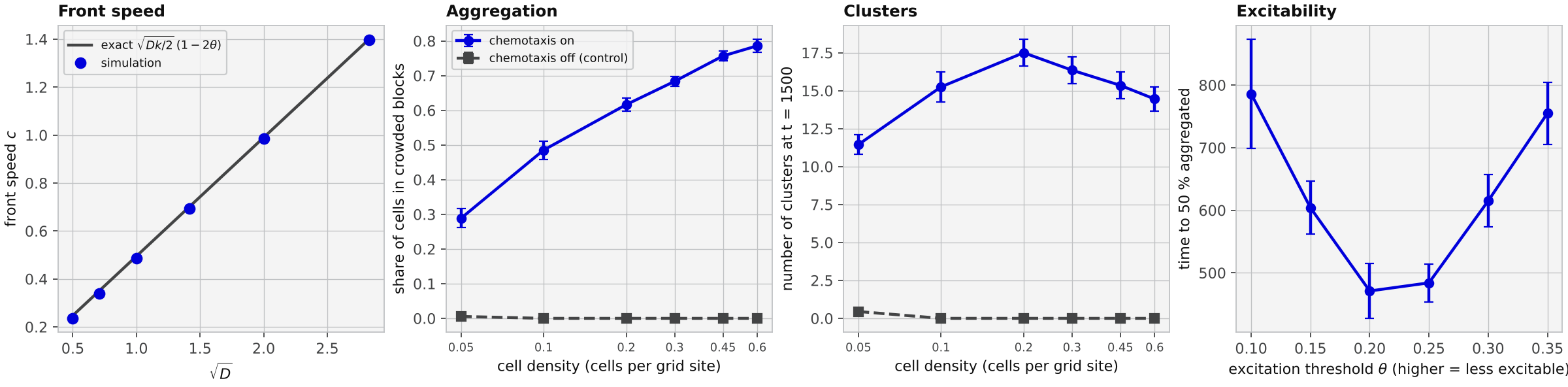{#fig-dicty-experiment fig-alt="Four panels. Panel one: front speed rises along a straight line from 0.24 to 1.40 as the square root of D goes from 0.5 to 2.8, simulation points on the exact line. Panel two: with chemotaxis the share of cells in crowded blocks rises from 0.29 at density 0.05 to 0.79 at density 0.6; without chemotaxis it stays at zero. Panel three: with chemotaxis the number of clusters rises from 11 at density 0.05 to 17.5 at 0.2 and falls to 14 at 0.6; without chemotaxis it is zero. Panel four: the time to reach 50 percent aggregated falls from about 790 at threshold 0.1 to about 470 at 0.2, stays near 480 at 0.25 and rises to about 755 at 0.35."}
```{python}
#| label: tbl-dicty-density
import csv
import numpy as np

rows = list(csv.DictReader(open("data/dicty_runs.csv")))
print("density  runs  reached 50 %  mean time to 50 %   share at 1500   clusters at 1500   (chemotaxis on)")
for d in (0.05, 0.1, 0.2, 0.3, 0.45, 0.6):
    sel = [r for r in rows if r["sweep"] == "density" and r["chemotaxis"] == "1" and float(r["value"]) == d]
    t = np.array([float(r["t_agg"]) for r in sel])
    sh = np.array([float(r["share"]) for r in sel])
    cl = np.array([float(r["clusters"]) for r in sel])
    hit = np.mean([float(r["aggregated"]) for r in sel])
    ci = lambda x: 1.96 * x.std(ddof=1) / np.sqrt(len(x))
    print(f"{d:6.2f}  {len(sel):4d}  {100 * hit:8.0f} %   {t.mean():8.0f} +- {ci(t):3.0f}      {sh.mean():6.2f} +- {ci(sh):4.2f}    {cl.mean():6.1f} +- {ci(cl):3.1f}")
```
What the figure shows:
- **The signal is needed.** With chemotaxis switched off, the waves still run (the number of firings is the same), but no crowded block forms: the share is 0.00 for every density from 0.1 to 0.6. This control is expected, since cells that walk at random do not crowd, but it shows that all aggregation in the model comes from the rising-front rule.
- **Denser populations aggregate faster and more completely.** The mean time to reach 50% falls from 1403 (density 0.1; only 8 of 20 runs got there, so this mean is cut off at 1500) to 891, 604, 450 and 345 time units at densities 0.2, 0.3, 0.45 and 0.6, and the share at 1500 rises from 0.29 to 0.79. At density 0.05 none of the 20 runs reached 50%. Part of this is a plain consequence of the setup: **the firing rate is per cell, so a denser dish also fires more often** (30 firings per run at density 0.05, 351 at density 0.6). I did not separate the effect of the density on the relay from the effect of the firing rate; that would need a run with a fixed total firing rate.
- **The number of clusters is not monotone in the density.** It rises from 11.4 at density 0.05 to 17.5 at 0.2 and falls to 14.4 at 0.6. With few cells there are too few cells to make a crowded block; at high density, neighbouring territories seem to merge. The second part is my reading of the pictures and I did not test it.
- **Excitability has a best value.** The time to 50% is 786 at $\theta = 0.1$, about 470 to 484 at 0.2 and 0.25, and 755 at 0.35, a U-shape, while the final share stays within 0.60 to 0.68. A possible reading is that a very excitable medium (low $\theta$) fires large waves that sweep the whole dish and leave less time for single territories, and that a hardly excitable medium (high $\theta$) has slow fronts (@eq-speed: $c \to 0$ at $\theta = 1/2$); I did not test this. The number of clusters rises from 13.2 to 20.4 as $\theta$ goes from 0.1 to 0.3.
- **The front speed obeys the square root law.** The simulated speed is within 5% of @eq-speed for every $D$ and within 1% for $D \ge 2$ (@fig-front-speed); the small deviation at low $D$ is the discreteness of the grid, because the front is only $\sqrt{2D/k} \approx 0.7$ sites wide at $D = 0.25$.
The wave period is not shown: I did not measure it in a way that I trust, because in the default dish the waves are a mixture of expanding rings and arcs without a regular source.
::: {.callout-note}
## Exercise 1: the front speed $c \sim \sqrt{Dk}$
(a) Use dimensional analysis on $u_t = D\,u_{xx} + k\,u(1-u)(u-\theta)$ to show that the front speed has the form $c = \sqrt{D k}\,F(\theta)$. (b) Find $F(\theta)$ exactly by inserting the front $u(x,t) = 1/(1 + e^{z/w})$ with $z = x - ct$ and an unknown width $w$. (c) By what factor must $D$ grow to double $c$? Check your answer against @fig-front-speed.
:::
::: {.callout-tip collapse="true"}
## Solution
(a) Write $x = \sqrt{D/k}\ \xi$ and $t = \tau/k$. Then $u_\tau = u_{\xi\xi} + u(1-u)(u-\theta)$, an equation with no parameters except $\theta$. Its front moves at a speed $F(\theta)$ in the units of $\xi$ per $\tau$, so in the original units $c = F(\theta)\,\sqrt{D/k}\cdot k = \sqrt{D k}\,F(\theta)$.
(b) With $u = (1 + e^{z/w})^{-1}$ we get $u_z = -u(1-u)/w$ and $u_{zz} = u(1-u)(1-2u)/w^2$. A travelling front has $u_t = -c\,u_z = (c/w)\,u(1-u)$. Insert this in the equation and divide by $u(1-u)$:
$$
\frac{c}{w} = \frac{D(1-2u)}{w^2} + k\,(u - \theta) = \Bigl(\frac{D}{w^2} - k\theta\Bigr) + u\Bigl(k - \frac{2D}{w^2}\Bigr).
$$
The left side does not depend on $u$, so the coefficient of $u$ must vanish: $w = \sqrt{2D/k}$. Then $c = w\,(D/w^2 - k\theta) = \sqrt{Dk/2} - \theta\sqrt{2Dk} = \sqrt{Dk/2}\,(1 - 2\theta)$, which is @eq-speed with $F(\theta) = (1-2\theta)/\sqrt 2$. For $\theta = 0.15$ and $D = k = 1$ this gives $c = 0.495$, and the simulation gives 0.487. The front has width $w = \sqrt{2D/k} \approx 1.4$ grid sites for $D = k = 1$, which is why the grid must not be coarser than that.
(c) $c \propto \sqrt D$, so doubling $c$ needs four times the diffusion coefficient. In @fig-front-speed the measured speed at $D = 4$ is twice that at $D = 1$ (0.986 and 0.487). Note also that $c = 0$ at $\theta = 1/2$ and that the front runs backward for $\theta > 1/2$: the medium is then no longer excitable.
:::
::: {.callout-note}
## Exercise 2: the stability limit of the explicit scheme
Show that the explicit Euler update with the five-point Laplacian is unstable for $\Delta t > \Delta x^2/(4D)$. (Hint: try the checkerboard mode $u_{ij} = (-1)^{i+j}$.) Then say what the limit would be on a grid with $\Delta x = 0.5$ and $D = 1$, and what it means for the cost of a simulation of fixed length when the grid is refined.
:::
::: {.callout-tip collapse="true"}
## Solution
For the checkerboard, every neighbour of a site has the opposite sign, so the sum of the four neighbour differences is $-4u_{ij} - 4u_{ij} = -8u_{ij}$. With only diffusion, one step multiplies the mode by $1 - 8D\,\Delta t/\Delta x^2$. Stability needs $|1 - 8D\,\Delta t/\Delta x^2| \le 1$, that is $\Delta t \le \Delta x^2/(4D)$. All other modes have smaller factors, so this one is the first to fail. (The reaction terms add only a small, bounded rate and do not change this limit in practice.) With $\Delta x = 0.5$ and $D = 1$ the limit is $0.0625$, four times smaller than for $\Delta x = 1$. Halving the grid spacing multiplies the number of sites by 4 and the number of time steps by 4, so the cost grows by a factor of 16. The `self_test()` confirms the limit: $D\,\Delta t = 0.2$ stays bounded and $D\,\Delta t = 0.4$ does not.
:::
::: {.callout-note}
## Exercise 3: why the cells only walk on rising fronts
Suppose a cell followed $\nabla u$ **all the time** (speed $v_\text{chem}$ whenever the gradient is non-zero). Explain why, for a symmetric wave pulse that passes the cell, the net displacement would be close to zero. Then compute how far a cell moves toward the source in one wave with the rule of @eq-cells and the default parameters, and how many waves a cell at distance 25 grid sites needs to reach a source.
:::
::: {.callout-tip collapse="true"}
## Solution
A pulse that moves away from its source has the cAMP **increasing** at the cell while the front passes, and then **decreasing** while the back passes. In the first phase $\nabla u$ points toward the source and in the second phase it points away from it. For a symmetric pulse the two phases last equally long, so a cell that follows the gradient all the time moves toward the source and then back by the same distance. Switching on the movement only while $\dot u > r$ keeps the first half and drops the second. With the default parameters the cell walks for $t_\text{chem} = 6$ time units at $v_\text{chem} = 0.3$, so it moves $0.3 \times 6 = 1.8$ grid sites toward the source per wave (if it keeps its heading; the heading noise makes it a little less). A cell at distance 25 needs at least $25/1.8 \approx 14$ waves. This is one reason why aggregation in the model takes hundreds of time units, and why more frequent firing speeds it up.
:::
::: {.python-next}
**Build this in Python.** Use `sweep` to vary the diffusion coefficient `D` or the recovery rate `eps`. Does the wave length (speed times period) change the size of the territories and so the number of clusters? Then change `rho_c` and find the cell density at which the medium stops carrying waves. Compare this value with the condition under which the cubic of @eq-field has an excited state when the degradation $\mu$ is added.
:::
## Biological reality check
How well does the model match what is known about *Dictyostelium*? The points below separate what the model keeps from what it leaves out.
**What matches.**
- *Waves with a refractory period.* The cAMP signal travels as waves that do not run back, because the cells that have just fired cannot fire again for a while. This is the relay logic of the receptor-based models [@martiel1987model] and of the cell-based excitable model [@palsson1996cell].
- *Cells move toward the source at the front.* Measurements report that cells move toward the wave source at the wave fronts [@ford2023spirals]; the rising-front rule of @eq-cells is a minimal version.
- *Aggregation territories.* In the cell-based model each aggregation centre has its own territory [@palsson1996cell]. In our model the same happens: each cluster sits at the centre of a patch that was emptied of cells.
- *The relay needs enough cells.* In the model, a dish with few cells carries waves poorly, which fits the idea that a critical density is needed.
**What is simplified or missing.**
- *The relay is coarse-grained.* There is no cell-level state: no receptor, no intracellular cAMP, no desensitisation. The recovery variable $v$ is a generic slow inhibitor of Barkley type, not the receptor desensitisation of the Martiel and Goldbeter model.
- *No sustained spirals.* Measured populations show spiral waves with periods between 3.5 and 5.5 min [@ford2023spirals]. In our default parameters I saw expanding rings and curved arcs, and one attempt to start a spiral by a cross-field initial condition did not give a rotating wave. The wave length is too long for a $100 \times 100$ dish. This is a limit of my parameter choice and not a proof that the model cannot make spirals; I did not search the parameters systematically.
- *No wave period in minutes.* Time is in units of $1/k$. I did not fit the model to any measured period, speed or cell speed, and the ratio between the speed of the wave and the speed of the cells is chosen so that aggregation happens in a few hundred time units; it is much less extreme in the model than I expect it to be in real cells, but I did not verify real numbers.
- *Point cells.* There is no volume, no adhesion and no cell-cell contact, so streams and clusters have no structure, and clusters can become very dense. Real cells also differ (some fire earlier than others), while all model cells have the same firing rate.
- *The firing is spontaneous and constant.* Cells fire at a fixed random rate from the start. In real populations, the onset of signalling comes with starvation and development, and it is not simply a random process.
- *Two dimensions only,* no cell division or death, no cell differentiation, no change in time of the parameters.
The honest summary is this: the model captures the *logic* of relay plus a rising-front ratchet, and it shows that this logic can gather a crowd into a few clusters without a leader. It does not support quantitative statements about real *Dictyostelium*.
## What this model does not do
- It is a **teaching model**. The parameters are not fitted to data, and the numbers in @fig-dicty-experiment should not be read as predictions for real cells.
- The relay is a **mean-field closure** (a relay capacity from the local density), not a cell-by-cell signalling model.
- The cells do **not adapt** to the cAMP level, are **points**, and do **not stick** to each other.
- The field has a **linear** degradation. The real extracellular cAMP is broken down by an enzyme (phosphodiesterase) that is itself regulated; the model has none of this dynamics.
- The dish has **no-flux walls** and a fixed size. A cluster in the model is a place where cells are crowded; it does not become a multicellular body.
- The **time to aggregate** and the **number of clusters** depend on the choices I made for $\rho_c$, $t_\text{chem}$, $v_\text{chem}$ and the firing rate. Change them and the numbers change.
- There are **no sustained spirals** in the default setting (see the reality check).
## References {.unnumbered}
The wave period of about 6 minutes sometimes quoted for *Dictyostelium* is not stated on this page, because it could not be verified. The title of Ford, Manhart and Chubb (2023) was written from memory and should be checked against the journal page before publication.
::: {#refs}
:::