---
title: "Triadic Closure"
subtitle: "Module 5: Complex Networks"
format: html
---
::: {.callout-note}
## Reading
- **Compulsory:** @holme2002growing for the original model (preferential attachment with triadic closure), and @newman2003structure, Section 3.2, for the definitions of the clustering coefficient. For the maximum-likelihood fit of the tail exponent used below, see Eq. (3.7) of @clauset2009power.
:::
The three models of [Comparing Graph Models](comparing-models.qmd) each reproduce one feature of real networks and miss another. The summary is
| Network | $L$ | $C$ | $p(k)$ |
|---|---|---|---|
| Real networks | small | high | heavy tail |
| Erdős-Rényi | $\sim \log N$ ✓ | low ✗ | Poisson ✗ |
| Watts-Strogatz | small ✓ | high ✓ | narrow ✗ |
| Barabási-Albert | very small ✓ | low ✗ | $k^{-3}$ ✓ |
One more ingredient closes the gap: **triadic closure**, the social rule "a friend of my friend becomes my friend". The model that adds it to preferential attachment is due to Holme and Kim [@holme2002growing].
## The model
The network grows as in the Barabási-Albert model: at each step a new node arrives with $m$ edges.
1. The first edge attaches by preferential attachment, to node $i$ with probability $\Pi_i = k_i / \sum_j k_j$. Call its target $w$.
2. For each of the other $m-1$ edges, with probability $p_t$ perform a **triad formation step**: connect the new node to a random neighbour of $w$, which closes a triangle $\text{new} - w - \text{neighbour}$. Otherwise attach by preferential attachment.
The triad probability is often written $p$; we write $p_t$ here to keep $p$ for the edge probability of the random graph. At $p_t = 0$ the model is the Barabási-Albert model, and for $m = 1$ there is no second edge, so no triangle can ever be created. NetworkX implements the model as `nx.powerlaw_cluster_graph(n, m, p)`. Its documentation points out one detail: if every neighbour of $w$ is already linked to the new node, the step falls back to preferential attachment.
## Clustering is tunable
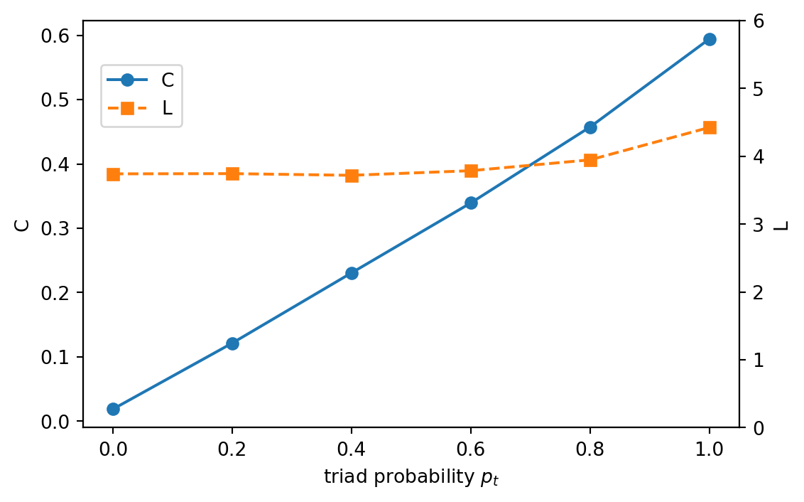
@fig-hk-clustering varies $p_t$ at fixed size.
```{python}
#| label: fig-hk-clustering
#| fig-cap: "Average clustering coefficient and average path length of the Holme-Kim graph (N = 2000, m = 3) as a function of the triad probability p_t, averaged over 4 graphs. The value at p_t = 0 is the Barabási-Albert graph. Clustering grows roughly linearly with p_t while the path length changes by less than 20%."
import matplotlib.pyplot as plt
import networkx as nx
import numpy as np
from scipy.sparse.csgraph import shortest_path

SEED = 7


def avg_path_length(G, n_src=300, seed=0):
    """Average distance in the largest component, from at most n_src random sources."""
    H = G.subgraph(max(nx.connected_components(G), key=len))
    nodes = list(H)
    A = nx.to_scipy_sparse_array(H, nodelist=nodes, format="csr")
    # SciPy's csgraph routines require int32 CSR index buffers in this environment.
    A.indices = A.indices.astype(np.int32)
    A.indptr = A.indptr.astype(np.int32)
    n = len(nodes)
    rng = np.random.default_rng(seed)
    src = np.arange(n, dtype=np.int32) if n <= n_src else rng.choice(n, n_src, replace=False).astype(np.int32)
    return shortest_path(A, unweighted=True, indices=src).sum() / (len(src) * (n - 1))


pts = np.linspace(0, 1, 6)
C_pt, L_pt = [], []
for pt in pts:
    graphs = [nx.powerlaw_cluster_graph(2000, 3, pt, seed=SEED + r) for r in range(4)]
    C_pt.append(np.mean([nx.average_clustering(G) for G in graphs]))
    L_pt.append(np.mean([avg_path_length(G) for G in graphs]))

fig, ax = plt.subplots(figsize=(6, 3.8))
ax.plot(pts, C_pt, "o-", label="C")
ax.set_xlabel(r"triad probability $p_t$")
ax.set_ylabel("C")
ax2 = ax.twinx()
ax2.plot(pts, L_pt, "s--", color="C1", label="L")
ax2.set_ylabel("L")
ax2.set_ylim(0, 6)
fig.legend(loc="upper left", bbox_to_anchor=(0.12, 0.88))
plt.tight_layout()
plt.show()
print("p_t:", np.round(pts, 2))
print("C  :", np.round(C_pt, 3))
print("L  :", np.round(L_pt, 2))
```
The maximum clustering for $m = 3$ is about 0.6, not 1. Only the edges after the first can close triangles, so at birth a new node with $m$ edges has about $m - 1$ closed pairs among its $m(m-1)/2$ neighbour pairs, a local clustering of about $2/m$ (0.67 for $m = 3$). This sets a ceiling well below 1. In other words the clustering is "finite": it does not decay with $N$, as the clustering figure in [Scaling of Path Length and Clustering](model-scaling.qmd) shows.
## The degree distribution is still scale-free
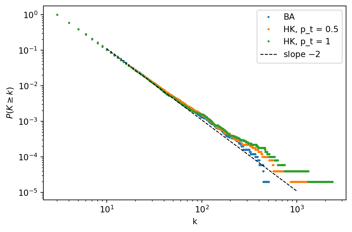
The additional step changes who is connected to the new node but not the rich-get-richer mechanism, so the tail should stay a power law with exponent close to 3. @fig-hk-degree compares the complementary cumulative distribution $P(K \ge k)$ of the Barabási-Albert and the Holme-Kim graphs. For $p(k) \sim k^{-\gamma}$ this distribution decays like $k^{-(\gamma - 1)}$, so a slope of $-2$ corresponds to $\gamma = 3$. The exponent is estimated with the maximum-likelihood formula for discrete data, $\hat\gamma \simeq 1 + n \big[\sum_{i} \ln \big(k_i / (k_{\min} - \tfrac12)\big)\big]^{-1}$, applied to the $n$ nodes with $k_i \ge k_{\min}$ [@clauset2009power, Eq. 3.7].
```{python}
#| label: fig-hk-degree
#| fig-cap: "Complementary cumulative degree distribution P(K >= k) of a Barabási-Albert graph and of Holme-Kim graphs with p_t = 0.5 and 1 (N = 50000, m = 3), on logarithmic axes. The dashed line has slope -2, which corresponds to p(k) ~ k^-3."
def gamma_mle(deg, kmin):
    x = deg[deg >= kmin]
    return 1 + len(x) / np.sum(np.log(x / (kmin - 0.5)))


graphs = {
    "BA": nx.barabasi_albert_graph(50_000, 3, seed=1),
    "HK, p_t = 0.5": nx.powerlaw_cluster_graph(50_000, 3, 0.5, seed=1),
    "HK, p_t = 1": nx.powerlaw_cluster_graph(50_000, 3, 1.0, seed=1),
}
fig, ax = plt.subplots(figsize=(6, 4))
for name, G in graphs.items():
    deg = np.array([d for _, d in G.degree()])
    ks = np.arange(3, deg.max() + 1)
    ccdf = np.array([(deg >= k).mean() for k in ks])
    ax.loglog(ks, ccdf, ".", ms=3, label=name)
    print(f"{name:>14}: k_max = {deg.max():5d}, gamma_hat(k_min = 10) = {gamma_mle(deg, 10):.2f}, "
          f"gamma_hat(k_min = 20) = {gamma_mle(deg, 20):.2f}, C = {nx.average_clustering(G):.3f}")
deg_ba = np.array([d for _, d in graphs["BA"].degree()])
ks = np.array([10, 1000])
ax.loglog(ks, (deg_ba >= 10).mean() * (ks / 10.0) ** -2, "k--", lw=1, label=r"slope $-2$")
ax.set_xlabel("k")
ax.set_ylabel(r"$P(K \geq k)$")
ax.legend()
plt.tight_layout()
plt.show()
```
The estimates are between 2.8 and 2.9 for all three graphs. They are below 3 because the formula is an approximation and because the finite sample and the discrete lower cutoff $k \ge m$ bias the estimate. The plain Barabási-Albert graph gives the same value, so the triad step does not change the exponent in a detectable way. For the Barabási-Albert model, @barabasi1999emergence report a simulated exponent of $2.9 \pm 0.1$ against the analytical value 3, which is consistent with these estimates.
## The completed comparison
@tbl-compare-models puts numbers in the summary table. All model graphs have $N = 5000$ and mean degree 6. The two real networks are the ones used in [Practice: Real Networks](practice-real-networks.qmd) and [Practice: Flights and Other Networks](practice-flights-network.qmd); they are small and, in the flights case, not connected, so $L$ is computed on the largest component.
```{python}
#| label: tbl-compare-models
#| tbl-cap: "Measured properties of the model graphs (N = 5000, mean degree 6, one graph each) and of two real networks. C_random = <k>/N is the clustering of a random graph with the same N and mean degree. kmax/<k> measures how far the degree distribution extends beyond its mean."
import gzip

N = 5000
models = {
    "Erdős-Rényi": nx.fast_gnp_random_graph(N, 6 / (N - 1), seed=1),
    "Watts-Strogatz (p = 0.1)": nx.watts_strogatz_graph(N, 6, 0.1, seed=1),
    "Barabási-Albert (m = 3)": nx.barabasi_albert_graph(N, 3, seed=1),
    "Holme-Kim (m = 3, p_t = 0.5)": nx.powerlaw_cluster_graph(N, 3, 0.5, seed=1),
}
enron = nx.Graph(nx.read_edgelist("data/ia-enron-only/ia-enron-only.edges"))
flights = nx.Graph(nx.read_graphml("data/openflights/openflights_usa.graphml.gz"))
rows = {**models, "Enron e-mail (data)": enron, "US flights (data)": flights}

print(f"{'network':<30}{'N':>6}{'<k>':>7}{'L':>6}{'C':>8}{'C/C_random':>12}{'kmax/<k>':>10}")
for name, G in rows.items():
    G.remove_edges_from(nx.selfloop_edges(G))
    k = np.array([d for _, d in G.degree()], dtype=float)
    C = nx.average_clustering(G)
    print(f"{name:<30}{len(G):>6}{k.mean():>7.1f}{avg_path_length(G):>6.2f}{C:>8.3f}{C / (k.mean() / len(G)):>12.1f}{k.max() / k.mean():>10.1f}")
```
Only the Holme-Kim row has all three properties of the real rows at once: short paths, an absolute clustering of the same order as the real values (0.27 against 0.43 and 0.49) and a degree distribution that extends far beyond its mean. The ratio $C/C_{\text{random}}$ alone is misleading, because $C_{\text{random}}$ depends on $N$: the plain Barabási-Albert graph has a ratio of 7, like the Enron network, but its clustering of 0.009 is not high in absolute terms. Two reservations apply. First, the conclusion is that these are only three features: degree assortativity, community structure and edge dynamics are not reproduced. The real networks of this table have negative degree correlations (flights) or none (Enron), a feature that none of the four models is built to produce. Second, a clustering far above $C_{\text{random}}$ is partly a consequence of the degree heterogeneity; the next page quantifies how much with a null model that keeps the degrees.
::: {.callout-note}
## Exercise
Generate Holme-Kim graphs with $N = 2000$ and $m = 1, 2, 3$ for $p_t = 1$ and compute their clustering coefficient. Explain the value for $m = 1$. Is the clustering larger for $m = 2$ or for $m = 3$, and why?
:::
::: {.callout-tip collapse="true"}
## Solution
```python
for m in (1, 2, 3):
    C = np.mean([nx.average_clustering(nx.powerlaw_cluster_graph(2000, m, 1.0, seed=s)) for s in range(4)])
    print(m, round(C, 3))
```
For $m = 1$ each new node has a single edge, so the graph is a tree and has no triangle at all: the clustering is zero. The measured values are 0, about 0.75 for $m = 2$ and about 0.59 for $m = 3$, so the clustering *decreases* with $m$. For $p_t = 1$ every edge after the first closes a triangle with the first target $w$, so a new node of degree $m$ is joined to $w$ and to $m-1$ neighbours of $w$. Its $m(m-1)/2$ neighbour pairs contain at least the $m-1$ pairs $(w, x)$, so its local clustering is at least $2/m$: 1 for $m = 2$ and 2/3 for $m = 3$. Larger $m$ means more neighbour pairs that triadic closure does not close.
:::
::: {.callout-note}
## Exercise
The Barabási-Albert graph and the Holme-Kim graph with $p_t = 1$ have almost the same exponent. Compute $\langle k^2 \rangle / \langle k \rangle$ for both graphs of @fig-hk-degree and use the heterogeneous mean-field threshold $\lambda_c = \langle k \rangle/\langle k^2 \rangle$ of [Epidemic Threshold](epidemic-threshold.qmd) to compare the predictions for SIS spreading. What does the prediction ignore?
:::
::: {.callout-tip collapse="true"}
## Solution
```python
for name, G in graphs.items():
    k = np.array([d for _, d in G.degree()], dtype=float)
    print(name, round(k.mean() / (k**2).mean(), 4))
```
With $N = 50000$ the prediction is $\langle k \rangle/\langle k^2 \rangle \approx 0.048$ for the Barabási-Albert graph, 0.030 for $p_t = 0.5$ and 0.020 for $p_t = 1$. The Holme-Kim graphs have a larger $\langle k^2 \rangle$ (their largest hubs are bigger, see the $k_{\max}$ printed above), hence a smaller predicted threshold. The mean-field formula uses only $p(k)$. It assumes that the network is uncorrelated and locally tree-like, so it ignores the triangles that triadic closure adds: edges inside a triangle transmit the infection to nodes that may already be infected. @pastor2015epidemic discuss the effect of short loops on epidemic thresholds.
:::
## What's Next?
[Configuration Model](configuration-model.qmd) shows how to separate the effect of the degree sequence from the effect of clustering.