Gray-Scott Model
Module 4: Space and Pattern Formation
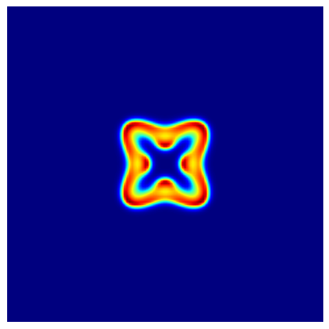
The Gray-Scott model combines diffusion with an autocatalytic reaction and produces spots, stripes, worms, and labyrinths depending on the parameters (Gray and Scott 1984; Pearson 1993).
This page follows the 2D Gierer-Meinhardt solver, and the jump is small.
- The domain is still a rectangular 2D grid.
- The Laplacian is still the vectorized 5-point stencil.
- Time stepping is still explicit Euler.
- The new ingredient is the reaction term, which is short to write and produces richer patterns.
- The main numerical change is the boundary condition: you keep the periodic wrapping built into
np.roll()instead of overwriting the edges with Neumann data.
The PDE system is
\[ \begin{aligned} \frac{\partial u}{\partial t} &= d_1 \Delta u - u v^2 + f(1-u), \\ \frac{\partial v}{\partial t} &= d_2 \Delta v + u v^2 - (f+k) v, \end{aligned} \tag{1}\]
where \(d_1\) and \(d_2\) are the diffusion coefficients, \(f\) is the feed rate, and \(k\) is the kill rate.
Start from the Homogeneous State
Gray-Scott is usually initialized near the steady state \((u, v) = (1, 0)\), then a small patch is perturbed.
Exercise
Set \(u = 0.5\), \(v = 0.25\) on a central square and add 10% noise there.
import numpy as np

n = 250
dt = 2.0
uv = np.ones((2, n, n), dtype=np.float32)
uv[1] = 0.0

c = n // 2
r = 12

# TODO: perturb a square patch around the center
# Set u close to 0.5 and v close to 0.25 in that patch

# TODO: add 10% Gaussian noise inside the same patch
Solution
uv[0, c - r : c + r, c - r : c + r] = 0.5
uv[1, c - r : c + r, c - r : c + r] = 0.25

noise = 0.1 * np.random.randn(2, 2 * r, 2 * r)
uv[:, c - r : c + r, c - r : c + r] *= 1 + noise
Reuse the 2D Laplacian
Exercise
We will start with the 5-point stencil. If you implemented the previous page cleanly, you can reuse that helper almost unchanged.
import numpy as np

def laplacian(field):
    # TODO: write the 5-point stencil with np.roll
    return lap
Solution
def laplacian(field):
    lap = -4 * field
    lap += np.roll(field, shift=1, axis=0)
    lap += np.roll(field, shift=-1, axis=0)
    lap += np.roll(field, shift=1, axis=1)
    lap += np.roll(field, shift=-1, axis=1)
    return lap
The only reason this already enforces periodic boundary conditions is that np.roll() wraps the array. If you wanted zero-flux or fixed-value boundaries here, you would keep the same Laplacian helper and reuse the boundary-update pattern from the 2D Gierer-Meinhardt page after every Euler step.
Implement the Gray-Scott PDE
Exercise
Write the Gray-Scott right-hand side from Equation 1.
import numpy as np

def gray_scott_pde(t, uv, d1=0.1, d2=0.05, f=0.040, k=0.060):
    u, v = uv
    lu = laplacian(u)
    lv = laplacian(v)

    # TODO: compute the autocatalytic term uv^2
    uv2 =

    # TODO: write du_dt and dv_dt
    du_dt =
    dv_dt =
    return np.array([du_dt, dv_dt])
Solution
def gray_scott_pde(t, uv, d1=0.1, d2=0.05, f=0.040, k=0.060):
    u, v = uv
    lu = laplacian(u)
    lv = laplacian(v)
    uv2 = u * v * v

    du_dt = d1 * lu - uv2 + f * (1 - u)
    dv_dt = d2 * lv + uv2 - (f + k) * v
    return np.array([du_dt, dv_dt])
Tip
Reference code is available in amlab/pdes_2d/gray_scott.py.
References
Gray, Peter, and Stephen K. Scott. 1984. “Autocatalytic Reactions in the Isothermal, Continuous Stirred Tank Reactor: Isolas and Other Forms of Multistability.” Chemical Engineering Science 39 (6): 1087–97. https://doi.org/10.1016/0009-2509(84)87017-7.
Pearson, John E. 1993. “Complex Patterns in a Simple System.” Science 261 (5118): 189–92. https://doi.org/10.1126/science.261.5118.189.