Michaelis-Menten Kinetics
Module 1: Low-Dimensional Dynamics
Optional extension
This page is optional. It applies the Session 3 workflow to a second rate law, with saturation instead of bistability.
Michaelis-Menten kinetics is one of the standard examples of a saturating nonlinear rate law (Michaelis and Menten 1913). The classical instantaneous rate is
\[ v(s) = \frac{V_{\max} s}{K_m + s}, \]
where \(V_{\max}\) is the maximum rate and \(K_m\) is the Michaelis constant.
In the reference script used in this course, the same saturating expression is reused as a simple teaching ODE,
\[ \dot s = \frac{V_{\max}s}{K_m + s} \tag{1}\]
This is not a full enzyme-substrate mass-action model. It is a compact one-dimensional example that lets you study how saturation changes both the rate curve and the time evolution of the state variable.
Small and Large Concentration Regimes
The rate law has two useful asymptotic regimes:
\[ v(s) \approx \frac{V_{\max}}{K_m} s \quad \text{for } s \ll K_m, \qquad v(s) \approx V_{\max} \quad \text{for } s \gg K_m. \]
So the system is approximately linear at small \(s\) and nearly constant-rate at large \(s\).
Implement the Saturating Rate Law
Exercise
Complete the right-hand side of the teaching ODE Equation 1.
def michaelis_menten(t, s, vmax=1.0, km=0.5):
    dsdt = # TODO: saturating rate law
    return dsdt
Solution
def michaelis_menten(t, s, vmax=1.0, km=0.5):
    """Saturating teaching ODE ds/dt = vmax * s / (km + s)."""
    return (vmax * s) / (km + s)
Reference Implementation
See:
amlab/odes_1d/michaelis_menten.py
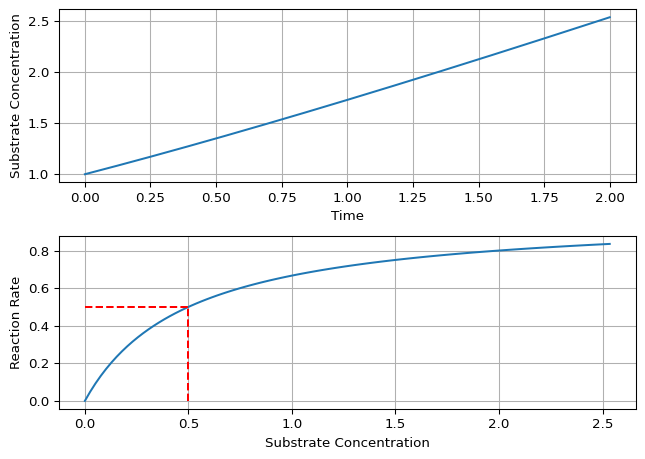
The helper plot_michaelis_menten(...) produces:
- \(s(t)\) over time
- \(v(s)\) with guides at \(s=K_m\) and \(v=V_{\max}/2\)
Render-time Figure
Interpret the Parameters
- Increasing \(V_{\max}\) raises the saturation plateau.
- Increasing \(K_m\) shifts the curve so larger values of \(s\) are needed before the rate is close to saturation.
- In the teaching ODE used here, larger \(V_{\max}\) also makes the state variable evolve faster in time.
Exploration
Exercise
Use plot_michaelis_menten to answer both questions.
- Increase \(V_{\max}\) and observe how the rate curve changes.
- Increase \(K_m\) (lower affinity). How does the saturation point shift?
Solution
Doubling \(V_{\max}\) doubles \(v(s)\) at every \(s\): the plateau rises and the half-saturation level \(V_{\max}/2\) rises with it, but it is still reached at \(s = K_m\). Increasing \(K_m\) moves the half-saturation point to the right, so you need a larger \(s\) before the rate is close to \(V_{\max}\). The initial slope \(V_{\max}/K_m\) falls.
import numpy as np

from amlab.odes_1d.michaelis_menten import michaelis_menten

s = np.array([0.5, 1.0, 5.0])
for vmax, km in [(1.0, 0.5), (2.0, 0.5), (1.0, 2.0)]:
    print(f"vmax={vmax}, km={km}: v(s) = {np.round(michaelis_menten(0, s, vmax, km), 3)}")
vmax=1.0, km=0.5: v(s) = [0.5 0.667 0.909]
vmax=2.0, km=0.5: v(s) = [1. 1.333 1.818]
vmax=1.0, km=2.0: v(s) = [0.2 0.333 0.714]Run Locally
python amlab/odes_1d/michaelis_menten.pyLimitations
In the classical mechanism the substrate is consumed, so \(s\) decreases. The teaching ODE above has a positive rate and makes \(s\) grow without bound. Use it only to study the shape of the saturating law, not as a model of an enzyme reaction.
Next
Michaelis, Leonor, and Maud L. Menten. 1913. “Die Kinetik Der Invertinwirkung.” Biochemische Zeitschrift 49: 333–69.