---
title: "Fitting Power Laws Properly"
subtitle: "Module 3: Modelling with Randomness"
format: html
---
::: {.callout-note}
## Reading
- **Compulsory:** @clauset2009power, Sections 1 to 5 and Box 1.
- **Recommended:** @newman2005power.
:::
[Power Laws](power-laws.qmd) explained why a straight line on a log-log plot is a weak argument and gave the maximum likelihood estimator for a known $x_{\min}$. In practice $x_{\min}$ is unknown, and a fitted exponent says nothing about whether the power law is a good model. On this page you implement the complete procedure of @clauset2009power on synthetic data whose true distribution you know. You then know what a correct answer looks like before you apply the procedure to returns in the [Tail Exponent](tail-exponent.qmd) lab.
## The recipe
@clauset2009power summarise their method in three steps (their Box 1).
1. **Fit.** Estimate $\alpha$ by maximum likelihood for every candidate $x_{\min}$ and choose the $x_{\min}$ that minimizes the Kolmogorov-Smirnov distance between the data above $x_{\min}$ and the fitted power law.
2. **Test the fit.** Compute a p-value for the power-law hypothesis with a Monte Carlo procedure. The authors treat the power law as ruled out if $p \le 0.1$ and as plausible if $p > 0.1$. A large $p$ does not prove the power law, and with few data a large $p$ is easy to obtain.
3. **Compare alternatives.** Compare the power law with other distributions (log-normal, exponential, stretched exponential, power law with cutoff) through a log-likelihood ratio and its significance.
The limits of each step matter as much as the steps. The maximum likelihood estimate is unbiased only for large samples, and the authors suggest that $n \gtrsim 50$ tail observations give a reasonably reliable estimate. Their KS-based choice of $x_{\min}$ worked well in their tests once roughly 1000 or more observations lay above $x_{\min}$, and it is a procedure with no performance guarantee [@clauset2009power, Sections 3.2 to 3.4].
## Step 1: choosing $x_{\min}$
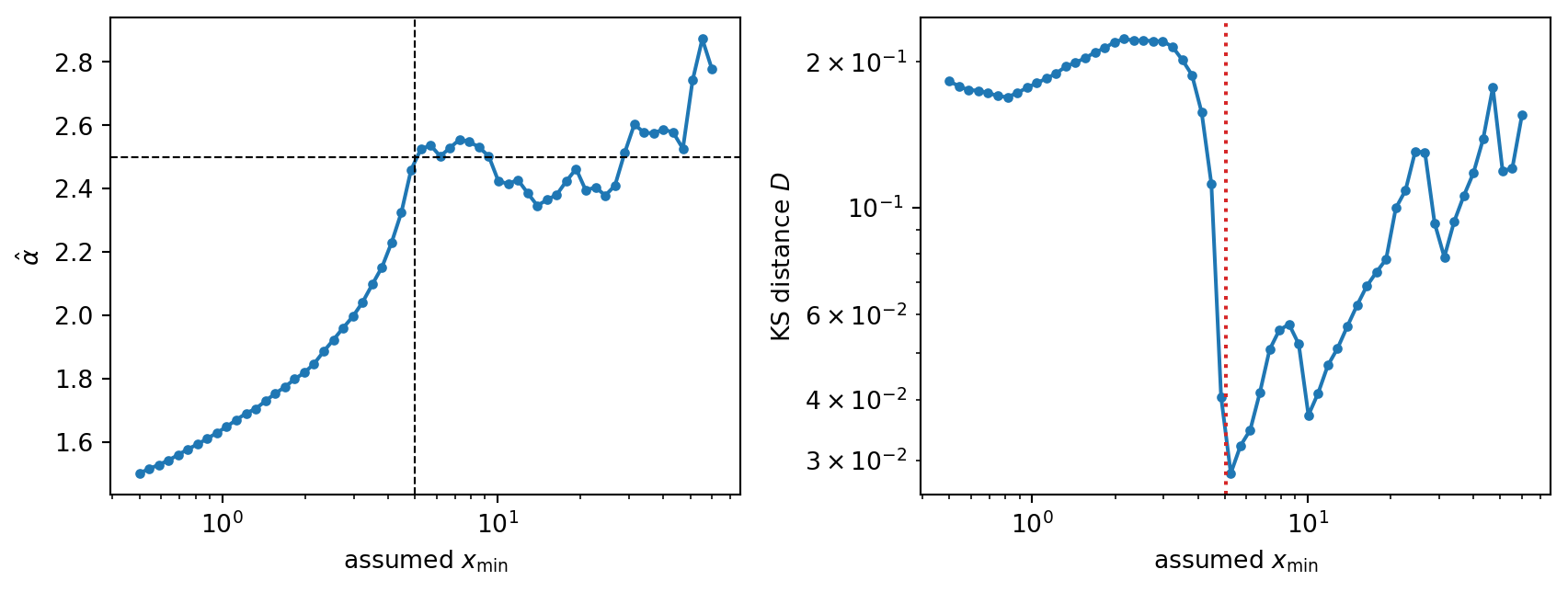
Take an assumed $x_{\min}$ that is too low, and the fit includes data that do not follow the power law, so $\hat{\alpha}$ is biased. Take it too high, and you discard legitimate data, so the statistical error grows. The figure shows both effects for a sample that follows a power law above $x_{\min} = 5$ and has an exponential body below.
```{python}
#| label: fig-xmin-scan
#| fig-cap: "Left: maximum likelihood estimate of $\\alpha$ against the assumed $x_{\\min}$ for 2000 samples that follow a power law with $\\alpha = 2.5$ above $x_{\\min} = 5$ and an exponential body below (dashed lines: true values). Right: KS distance between the data above the assumed $x_{\\min}$ and the fitted power law. The vertical dotted line marks the $x_{\\min}$ with the smallest distance."
import time

import matplotlib.pyplot as plt
import numpy as np
from scipy import optimize, special


def sample_power_law(n, alpha, xmin, rng):
    """Inverse-transform samples of p(x) = (alpha - 1) / xmin * (x / xmin)^(-alpha), x >= xmin."""
    return xmin * (1.0 - rng.random(n)) ** (-1.0 / (alpha - 1.0))


def sample_with_body(n, alpha, xmin, rng, share_tail=0.4, scale=2.0):
    """Power law above xmin, exponential body (scale `scale`) truncated at xmin below."""
    k = rng.binomial(n, share_tail)
    u = rng.random(n - k)
    body = -scale * np.log(1.0 - u * (1.0 - np.exp(-xmin / scale)))
    return np.concatenate([sample_power_law(k, alpha, xmin, rng), body])


def ks_distance(tail, xmin, alpha):
    """KS distance between the empirical CDF of `tail` and the fitted power law."""
    xs = np.sort(tail)
    n = xs.size
    model = 1.0 - (xs / xmin) ** (1.0 - alpha)
    return max((np.arange(1, n + 1) / n - model).max(), (model - np.arange(n) / n).max())


def fit_at(x, xmin):
    """MLE of alpha and KS distance for the data with x >= xmin."""
    tail = x[x >= xmin]
    alpha = 1.0 + tail.size / np.sum(np.log(tail / xmin))
    return alpha, ks_distance(tail, xmin, alpha)


def fit_power_law(x, n_tail_min=50, max_candidates=100):
    """Maximum likelihood fit with xmin chosen by minimizing the KS distance.

    Candidates are data values that leave at least `n_tail_min` points above;
    for speed at most `max_candidates` of them are scanned (a coarse grid of
    quantiles). Clauset et al. scan every observed value.
    """
    x = np.sort(np.asarray(x, dtype=float))
    pool = np.unique(x[: x.size - n_tail_min])
    if pool.size > max_candidates:
        pool = np.unique(np.quantile(pool, np.linspace(0, 1, max_candidates)))
    best = None
    for xm in pool:
        alpha, d = fit_at(x, xm)
        if best is None or d < best["D"]:
            best = {"xmin": xm, "alpha": alpha, "D": d, "n_tail": int(np.sum(x >= xm))}
    best["se"] = (best["alpha"] - 1.0) / np.sqrt(best["n_tail"])
    return best


rng = np.random.default_rng(2009)
x = sample_with_body(2000, 2.5, 5.0, rng)
scan = np.logspace(np.log10(0.5), np.log10(60), 60)
alphas, dists = np.array([fit_at(x, xm) for xm in scan]).T
chosen = fit_power_law(x)

fig, axes = plt.subplots(1, 2, figsize=(9, 3.5))
axes[0].semilogx(scan, alphas, "o-", ms=3)
axes[0].axhline(2.5, color="k", ls="--", lw=0.8)
axes[0].axvline(5.0, color="k", ls="--", lw=0.8)
axes[0].set_ylabel(r"$\hat{\alpha}$")
axes[1].loglog(scan, dists, "o-", ms=3)
axes[1].axvline(chosen["xmin"], color="C3", ls=":")
axes[1].set_ylabel("KS distance $D$")
for ax in axes:
    ax.set_xlabel("assumed $x_{\\min}$")
plt.tight_layout()
plt.show()

print(f"KS choice: xmin = {chosen['xmin']:.2f}, alpha = {chosen['alpha']:.3f} +/- {chosen['se']:.3f} "
      f"(n_tail = {chosen['n_tail']}; true values 5 and 2.5)")
```
The estimate $\hat{\alpha}$ drifts away from the true value below $x_{\min} = 5$ and becomes noisy above it, which is the behaviour described by @clauset2009power in their Fig. 3.3. The KS distance is smallest close to the true $x_{\min}$. The selected value is not exact, because the scan uses a coarse grid and the sample is finite.
## Step 2: a goodness-of-fit p-value
The KS distance $D$ of the fit measures how far the data are from the fitted power law, but its distribution under the null hypothesis is unknown, because $x_{\min}$ and $\alpha$ were estimated from the same data. This is the same problem as with the normal fit in [Calibrated KS Test](ks-bootstrap.qmd), and @clauset2009power [footnote 7] give it as the reason for a Monte Carlo p-value. The procedure is:
1. Generate a synthetic data set of the same size. Draw each value from the fitted power law above $\hat{x}_{\min}$ with probability $n_{\text{tail}}/n$. Otherwise resample one of the observed values below $\hat{x}_{\min}$. This keeps the non-power-law body of the data.
2. Fit the synthetic set from scratch, including its own $x_{\min}$, and record its KS distance.
3. The p-value is the fraction of synthetic distances at least as large as the observed one.
The authors' rule of thumb is that a p-value accurate to $\epsilon$ needs at least $\tfrac{1}{4}\epsilon^{-2}$ synthetic sets. For $\epsilon = 0.01$ this is 2500. The code below uses 200 to keep the page fast, so its p-values are accurate to about $\pm 0.035$.
```{python}
def gof_p_value(x, fit, n_boot, rng):
    """Semiparametric bootstrap p-value (Clauset et al. 2009, Section 4.1)."""
    x = np.asarray(x, dtype=float)
    body = x[x < fit["xmin"]]
    share = fit["n_tail"] / x.size
    d_boot = np.empty(n_boot)
    for b in range(n_boot):
        k = rng.binomial(x.size, share)
        synthetic = np.concatenate([sample_power_law(k, fit["alpha"], fit["xmin"], rng),
                                    rng.choice(body, x.size - k)])
        d_boot[b] = fit_power_law(synthetic)["D"]  # refit xmin and alpha every time
    return np.mean(d_boot >= fit["D"])


print(f"synthetic sets needed for epsilon = 0.01: {0.25 / 0.01**2:.0f}")
print(f"accuracy of p with 200 sets: {np.sqrt(0.25 / 200):.3f}")
```
## Step 3: alternatives
A good fit of the power law does not exclude that another distribution fits as well. For two models with densities $p_1$ and $p_2$ fitted to the same tail data, the log-likelihood ratio is
$$
R = \sum_{i=1}^{n} \left[ \ln p_1(x_i) - \ln p_2(x_i) \right].
$$ {#eq-llr}
$R > 0$ favours model 1. Because $R$ fluctuates from sample to sample, its sign is only trustworthy if $R$ is significantly different from zero. @clauset2009power (Appendix C, following Vuong) approximate the fluctuations of $R$ by a normal law with variance $n\sigma^2$, where $\sigma^2$ is the variance of the pointwise differences. The p-value is
$$
p = \operatorname{erfc}\!\left( \frac{|R|}{\sqrt{2n}\,\sigma} \right).
$$ {#eq-vuong}
If $p$ is small, say below 0.1, the sign of $R$ is reliable. If $p$ is large the data do not discriminate between the two models, and the authors point out that this is itself a useful answer. This version of the test is for non-nested models. For a power law against a power law with cutoff, which are nested, the paper describes a modified test that this page does not implement.
All models are fitted on the tail $x \ge \hat{x}_{\min}$ only, so each density is normalized on that range.
```{python}
def tail_log_likelihoods(tail, xmin, alpha):
    """Pointwise log-likelihoods of power law, truncated log-normal and shifted exponential."""
    ll_power = np.log((alpha - 1.0) / xmin) - alpha * np.log(tail / xmin)
    lam = 1.0 / np.mean(tail - xmin)
    ll_exp = np.log(lam) - lam * (tail - xmin)
    lx = np.log(tail)

    def log_normal_ll(p):
        mu, s = p[0], np.exp(p[1])
        mass = 0.5 * special.erfc((np.log(xmin) - mu) / (s * np.sqrt(2.0)))
        return -lx - np.log(s * np.sqrt(2.0 * np.pi)) - (lx - mu) ** 2 / (2 * s**2) - np.log(mass)

    res = optimize.minimize(lambda p: -log_normal_ll(p).sum(),
                            [lx.mean(), np.log(lx.std())], method="Nelder-Mead")
    return ll_power, log_normal_ll(res.x), ll_exp


def vuong(ll_a, ll_b):
    """Log-likelihood ratio R of Eq. (llr) and its p-value, Eq. (vuong)."""
    d = ll_a - ll_b
    return d.sum(), special.erfc(abs(d.sum()) / (np.sqrt(2 * d.size) * d.std()))
```
## Three test cases
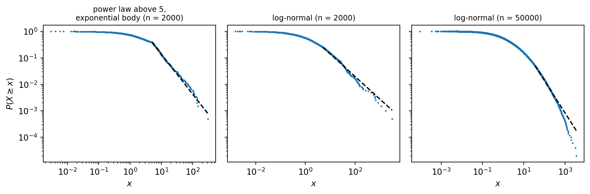
You now apply all three steps to three samples with known truth: a power law above 5 with an exponential body, a log-normal sample of 2000 values, and a log-normal sample of 50000 values. The log-normal has parameters $\mu = 0.3$ and $\sigma = 2$, the values @clauset2009power use to show that a log-normal looks straight on a log-log plot over a wide range.
```{python}
#| label: fig-three-cases
#| fig-cap: "Empirical CCDFs (dots) and maximum likelihood power laws above the selected $x_{\\min}$ (dashed lines) for the three synthetic samples. The log-normal curves bend downwards beyond the fitted line, but only a large sample makes this bend statistically visible."
rng = np.random.default_rng(2009)
samples = {
    "power law above 5,\nexponential body (n = 2000)": sample_with_body(2000, 2.5, 5.0, rng),
    "log-normal (n = 2000)": rng.lognormal(0.3, 2.0, 2000),
    "log-normal (n = 50000)": rng.lognormal(0.3, 2.0, 50000),
}

fig, axes = plt.subplots(1, 3, figsize=(10, 3.4), sharey=True)
t0 = time.time()
for ax, (name, x) in zip(axes, samples.items()):
    fit = fit_power_law(x)
    p_fit = gof_p_value(x, fit, n_boot=200, rng=rng)
    tail = x[x >= fit["xmin"]]
    ll_power, ll_lognormal, ll_exp = tail_log_likelihoods(tail, fit["xmin"], fit["alpha"])
    r_ln, p_ln = vuong(ll_power, ll_lognormal)
    r_ex, p_ex = vuong(ll_power, ll_exp)
    print(name.replace("\n", " "))
    print(f"  xmin = {fit['xmin']:.1f}, alpha = {fit['alpha']:.2f} +/- {fit['se']:.2f}, "
          f"n_tail = {fit['n_tail']}, goodness-of-fit p = {p_fit:.2f}")
    print(f"  power law vs log-normal:  R = {r_ln:7.2f}, p = {p_ln:.3f}")
    print(f"  power law vs exponential: R = {r_ex:7.1f}, p = {p_ex:.1e}")

    xs = np.sort(x)
    ax.loglog(xs, 1.0 - np.arange(xs.size) / xs.size, ".", ms=2)
    grid = np.logspace(np.log10(fit["xmin"]), np.log10(xs[-1]), 50)
    ax.loglog(grid, fit["n_tail"] / x.size * (grid / fit["xmin"]) ** (1.0 - fit["alpha"]), "k--")
    ax.set_title(name, fontsize=9)
    ax.set_xlabel("$x$")
axes[0].set_ylabel(r"$P(X \geq x)$")
plt.tight_layout()
plt.show()
```
Read the output as the paper recommends. For the true power law the goodness-of-fit p-value is above 0.1 and the exponential is rejected with a huge $R$. The log-normal cannot be told apart from the power law: its $p$ is large, so the data do not choose between the two. For the log-normal sample of 2000 values the outcome depends on the draw. In 30 repeated draws (60 synthetic sets each) the power law was rejected at the 0.1 level in about half of the runs, so a non-rejection in a single run, which is common at this sample size, proves nothing. This is the warning of the paper that a large p-value does not establish a power law. For the large sample the power law is rejected, and the likelihood ratio favours the log-normal significantly.
::: {.callout-note}
## Exercise
Apply the three steps to the absolute log returns of the lab series, `a = np.abs(r - r.mean())`. Report $\hat{x}_{\min}$, $\hat{\alpha}$, the number of observations above $\hat{x}_{\min}$, the goodness-of-fit p-value, and the likelihood-ratio results against the log-normal and exponential. Convert $\hat{\alpha}$ to the tail index of $\Pr(|r| > x)$ and compare it with the Hill estimate of [Tail Exponent](tail-exponent.qmd). Which assumption of the method do volatility clustering and the synthetic fallback series put at risk?
:::
::: {.callout-tip collapse="true"}
## Solution
The density exponent $\hat{\alpha}$ and the tail index $\alpha_{\text{tail}}$ of $\Pr(|r| > x) \sim x^{-\alpha_{\text{tail}}}$ are related by $\alpha_{\text{tail}} = \hat{\alpha} - 1$.
```{python}
from amlab.finance import load_prices, log_returns

r = log_returns(load_prices()["close"])
a = np.abs(r - r.mean())
rng = np.random.default_rng(5)

fit = fit_power_law(a, n_tail_min=100)
p_fit = gof_p_value(a, fit, n_boot=100, rng=rng)
tail = a[a >= fit["xmin"]]
ll_power, ll_lognormal, ll_exp = tail_log_likelihoods(tail, fit["xmin"], fit["alpha"])
print(f"xmin = {fit['xmin']:.4f}, alpha = {fit['alpha']:.2f} +/- {fit['se']:.2f}, "
      f"tail index = {fit['alpha'] - 1:.2f}, n_tail = {fit['n_tail']}, p = {p_fit:.2f}")
for name, ll in [("log-normal", ll_lognormal), ("exponential", ll_exp)]:
    R, p = vuong(ll_power, ll)
    print(f"power law vs {name}: R = {R:.2f}, p = {p:.3f}")
```
If $p \le 0.1$, the power law is rejected for this range. Otherwise it is plausible, which is a weaker statement than "the tail is a power law". For the likelihood ratios, a positive $R$ with a small $p$ favours the power law, a negative $R$ with a small $p$ favours the alternative, and a large $p$ means that the data cannot decide. Both the bootstrap and the Vuong test assume independent observations. Volatility clustering makes the effective number of independent observations smaller than $n_{\text{tail}}$, so the p-values are optimistic. If the series is the synthetic fallback of the lab, the result describes a GARCH simulation and not a market.
:::
## Limits of the method
- The three steps assume that the tail observations are independent and identically distributed. Return series are not, so treat p-values as indicative.
- The p-value is a tool for ruling a model out. Even a non-rejection is compatible with many other distributions, and the log-likelihood ratio can only compare the candidates you chose.
- The authors scan every observed value as a candidate for $x_{\min}$. The code above scans at most 100 quantiles of the data, which is faster and slightly coarser.
- The code handles continuous data. For integer data @clauset2009power give a different (discrete) maximum likelihood estimator and an approximation that replaces $x_{\min}$ by $x_{\min} - \tfrac{1}{2}$ in the estimator of [Power Laws](power-laws.qmd), which they report to be accurate to about 1 % for $x_{\min} \gtrsim 6$. Applying the continuous estimator to integer data is not recommended.