---
title: "Metapopulation Epidemics"
subtitle: "Module 5: Complex Networks"
format: html
---
::: {.callout-note}
## Reading
- **Compulsory:** @arenas2020modeling, Section II.B (social contacts and mobility among patches, Eqs. 12 to 19).
- **Recommended:** the same paper, Section III (effective reproduction number), and @barbeito2023effectiveness for the statistical counterpart (effect of restrictions on transmission in Spain).
- **Background:** [SIR Extensions](../low-dimensional-dynamics/sir-extensions.qmd) (Module 1), mobility matrix, and [The Final Size of an Epidemic](../low-dimensional-dynamics/final-size.qmd).
:::
So far in this module the nodes of the network were individuals. A network can also connect **populations**: cities, regions or countries, each with its own epidemic, linked by the movement of people. This is a **metapopulation** model. In the menu of extensions of [SIR Extensions](../low-dimensional-dynamics/sir-extensions.qmd) it is the row "a single population" replaced by "patches coupled by a mobility matrix". The mobility network does for whole populations what the contact network did for individuals: it decides **where and when** the infection arrives.
## The model
Consider $n$ patches, labelled $k = 1, \dots, n$, each with an SIR epidemic of its own, and a mobility matrix $m_{k\ell}$ that gives the rate at which individuals move from patch $k$ to patch $\ell$. For patch $k$,
$$
\begin{aligned}
\dot S_k &= -\beta_k S_k I_k + \sum_{\ell \neq k}\big(m_{\ell k} S_\ell - m_{k\ell} S_k\big), \\
\dot I_k &= \beta_k S_k I_k - \gamma_k I_k + \sum_{\ell \neq k}\big(m_{\ell k} I_\ell - m_{k\ell} I_k\big), \\
\dot R_k &= \gamma_k I_k + \sum_{\ell \neq k}\big(m_{\ell k} R_\ell - m_{k\ell} R_k\big).
\end{aligned}
$$ {#eq-metapop}
Susceptible, infected and recovered people all move with the same rates. The new behaviours are importation and exportation of cases and staggered regional waves, and a travel restriction is simply a change of the parameters in $m$.
To connect with the rest of the module, we take all patches to be identical ($\beta_k = \beta$, $\gamma_k = \gamma$) and the patches to form a graph with adjacency matrix $A$. Each individual leaves along each link of its patch at the same rate $\sigma$, so $m_{k\ell} = \sigma A_{k\ell}$. Then the sums in @eq-metapop become
$$
\sum_{\ell}\big(m_{\ell k} X_\ell - m_{k\ell} X_k\big) = \sigma \sum_\ell A_{k\ell}(X_\ell - X_k) = -\sigma\,(L X)_k,
\qquad L = D - A,
$$ {#eq-laplacian}
where $D$ is the diagonal matrix of degrees and $L$ is the **graph Laplacian**. The symmetric rates keep a uniform population uniform, so we can normalise each patch population to 1 and read $S_k, I_k, R_k$ as fractions. Mobility acts as diffusion on the graph, and the epidemic in each patch as a reaction term.
## Where and when does the epidemic arrive?
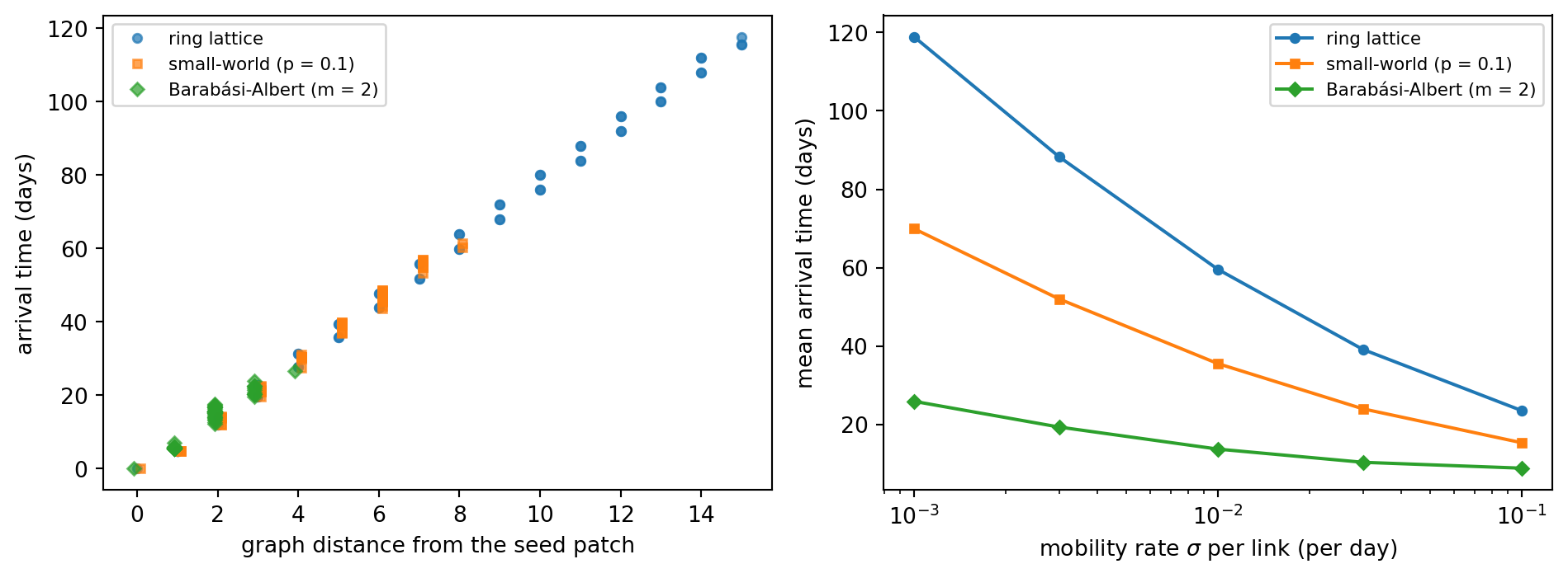
We start an outbreak in patch 0 (a fraction $10^{-3}$ of its population infected) and use $\beta = 0.3$ and $\gamma = 0.1$ per day, so that $R_0 = \beta/\gamma = 3$ in every patch, the value quoted by @arenas2020modeling for COVID-19. The **arrival time** of a patch is the first time at which its infected fraction exceeds $10^{-4}$. We compare three graphs of $n = 60$ patches with the same mean degree (about 4): a ring lattice in which each patch is joined to its 4 nearest neighbours, the same lattice with 10% of its links rewired (small-world, [Small-World Networks](small-world.qmd)), and a Barabási-Albert graph ([Preferential Attachment](preferential-attachment.qmd)).
```{python}
import matplotlib.pyplot as plt
import networkx as nx
import numpy as np
from scipy.integrate import solve_ivp
from scipy.stats import spearmanr

SEED = 7
beta, gamma = 0.3, 0.1


def simulate_patches(G, sigma, t_max=400, seed_patch=0, i0=1e-3, thr=1e-4):
    """Integrate the metapopulation SIR on the graph G of patches.

    Returns the arrival time of every patch, the solution and the population of every patch over time.
    """
    n = G.number_of_nodes()
    A = nx.to_numpy_array(G, nodelist=range(n))
    Lap = np.diag(A.sum(axis=1)) - A

    def rhs(t, y):
        S, I, R = y[:n], y[n:2 * n], y[2 * n:]
        return np.concatenate([-beta * S * I - sigma * Lap @ S,
                               beta * S * I - gamma * I - sigma * Lap @ I,
                               gamma * I - sigma * Lap @ R])

    y0 = np.concatenate([np.ones(n), np.zeros(n), np.zeros(n)])
    y0[seed_patch] -= i0
    y0[n + seed_patch] = i0
    t = np.linspace(0, t_max, 4001)
    sol = solve_ivp(rhs, (0, t_max), y0, t_eval=t, rtol=1e-8, atol=1e-12, method="LSODA")
    I = sol.y[n:2 * n]
    arrival = np.array([t[np.argmax(I[k] > thr)] if (I[k] > thr).any() else np.nan for k in range(n)])
    population = sol.y[:n] + sol.y[n:2 * n] + sol.y[2 * n:]
    return arrival, sol, population


n_patches = 60
patch_graphs = {
    "ring lattice": nx.watts_strogatz_graph(n_patches, 4, 0.0, seed=1),
    "small-world (p = 0.1)": nx.watts_strogatz_graph(n_patches, 4, 0.1, seed=1),
    "Barabási-Albert (m = 2)": nx.barabasi_albert_graph(n_patches, 2, seed=1),
}
sigma = 0.01
arrival = {}
print(f"{'patch graph':<26}{'<k>':>5}{'mean arrival':>14}{'last arrival':>14}{'Spearman(arrival, distance)':>29}{'max |N_k - 1|':>15}")
for name, G in patch_graphs.items():
    arr, sol, pop = simulate_patches(G, sigma)
    arrival[name] = arr
    dist = nx.single_source_shortest_path_length(G, 0)
    d = np.array([dist[k] for k in range(n_patches)])
    k_mean = 2 * G.number_of_edges() / n_patches
    print(f"{name:<26}{k_mean:>5.1f}{np.nanmean(arr):>14.1f}{np.nanmax(arr):>14.1f}"
          f"{spearmanr(d, arr)[0]:>29.3f}{np.abs(pop - 1).max():>15.1e}")
```
The last column is a check of the implementation: the population of every patch stays equal to 1 up to the integration error, as @eq-laplacian predicts for symmetric rates. The Spearman correlation between the arrival time and the number of links separating a patch from the seed is above 0.9 for all three graphs, so the arrival order is essentially the order of distance on the mobility network. The scale of the times, however, depends strongly on the topology: shortcuts and hubs bring the infection to every patch much earlier.
```{python}
#| label: fig-meta-arrival
#| fig-cap: "Metapopulation SIR on three graphs of 60 patches (R0 = 3 in every patch, mobility rate sigma per link). Left: arrival time of the infection in each patch (first time the infected fraction exceeds 1e-4) against its graph distance from the seed patch, for sigma = 0.01 per day. Right: mean arrival time over the patches against the mobility rate sigma. The time grows when mobility is restricted, with a slope that depends on the topology."
fig, axes = plt.subplots(1, 2, figsize=(10, 3.8))
for (name, G), marker in zip(patch_graphs.items(), "osD"):
    dist = nx.single_source_shortest_path_length(G, 0)
    d = np.array([dist[k] for k in range(n_patches)])
    axes[0].plot(d + 0.08 * (marker == "s") - 0.08 * (marker == "D"), arrival[name], marker, ms=4, alpha=0.7, label=name)
axes[0].set_xlabel("graph distance from the seed patch")
axes[0].set_ylabel("arrival time (days)")
axes[0].legend(fontsize=8)

sigmas = np.array([0.001, 0.003, 0.01, 0.03, 0.1])
for (name, G), marker in zip(patch_graphs.items(), "osD"):
    axes[1].semilogx(sigmas, [np.nanmean(simulate_patches(G, s, t_max=600)[0]) for s in sigmas], marker + "-", ms=4, label=name)
axes[1].set_xlabel(r"mobility rate $\sigma$ per link (per day)")
axes[1].set_ylabel("mean arrival time (days)")
axes[1].legend(fontsize=8)
plt.tight_layout()
plt.show()
```
::: {.callout-note}
## Exercise 1: hub or leaf
On the Barabási-Albert graph of patches, start the outbreak in the patch of largest degree and then in a patch of smallest degree. Compare the mean arrival times. What does this say about the importance of the place where an epidemic starts?
:::
::: {.callout-tip collapse="true"}
## Solution
```python
G = patch_graphs["Barabási-Albert (m = 2)"]
degs = dict(G.degree())
for label, seed_patch in [("hub", max(degs, key=degs.get)), ("leaf", min(degs, key=degs.get))]:
    arr = simulate_patches(G, 0.01, seed_patch=seed_patch)[0]
    print(label, degs[seed_patch], round(np.nanmean(arr), 1))
```
The seed in the hub reaches the other patches sooner than the seed in a leaf, since from the hub every other patch is a few links away and from a leaf the infection must first reach a hub; see the printed values. This is the same asymmetry between hubs and ordinary nodes that [Vaccination Strategies](vaccination-strategies.qmd) uses to design immunization.
:::
## A discrete-time mobility model
@arenas2020modeling use a different formalism, the *microscopic Markov chain approach*, in discrete time with one step per day. We keep its mobility ingredients and drop its age groups, ten compartments and density-dependent contacts, and use an SIR model. Each patch $i$ has $n_i$ residents. A fraction $p$ of them ("degree of mobility") commute, and a commuter from $i$ chooses patch $j$ with probability $R_{ij}$; here $R_{ij} = A_{ij}/k_i$. The *effective mobility matrix* is $M_{ji} = (1-p)\delta_{ji} + p R_{ji}$, the fraction of the residents of $j$ who are present in $i$, and the **effective population** of patch $i$ during the day is $\tilde n_i = \sum_j M_{ji} n_j$ [@arenas2020modeling, Eqs. 16 and 17]. With $\rho^I_j$ the infected fraction of the residents of $j$, a susceptible who is in patch $i$ is exposed to $\sum_j M_{ji} n_j \rho_j^I / \tilde n_i$ infected people per unit of the contacts it makes, so it is infected with probability
$$
P_i = 1 - (1-\beta_c)^{\bar k\, X_i}, \qquad X_i = \frac{\sum_j M_{ji}\, n_j\, \rho^I_j}{\tilde n_i},
$$ {#eq-mmca-P}
where $\beta_c$ is the probability of infection per contact and $\bar k$ the number of contacts. A resident of $i$ is infected with probability
$$
\Pi_i = (1-p)\,P_i + p\sum_j R_{ij}\,P_j,
$$ {#eq-mmca-Pi}
the first term for contagion in the home patch and the second for contagion in the patches visited [@arenas2020modeling, Eq. 12]. Then $\rho^S_i \leftarrow (1 - \Pi_i)\rho^S_i$, and the infected fraction gains $\Pi_i\rho^S_i$ and loses $\mu\rho^I_i$ per step.
```{python}
#| label: fig-meta-mmca
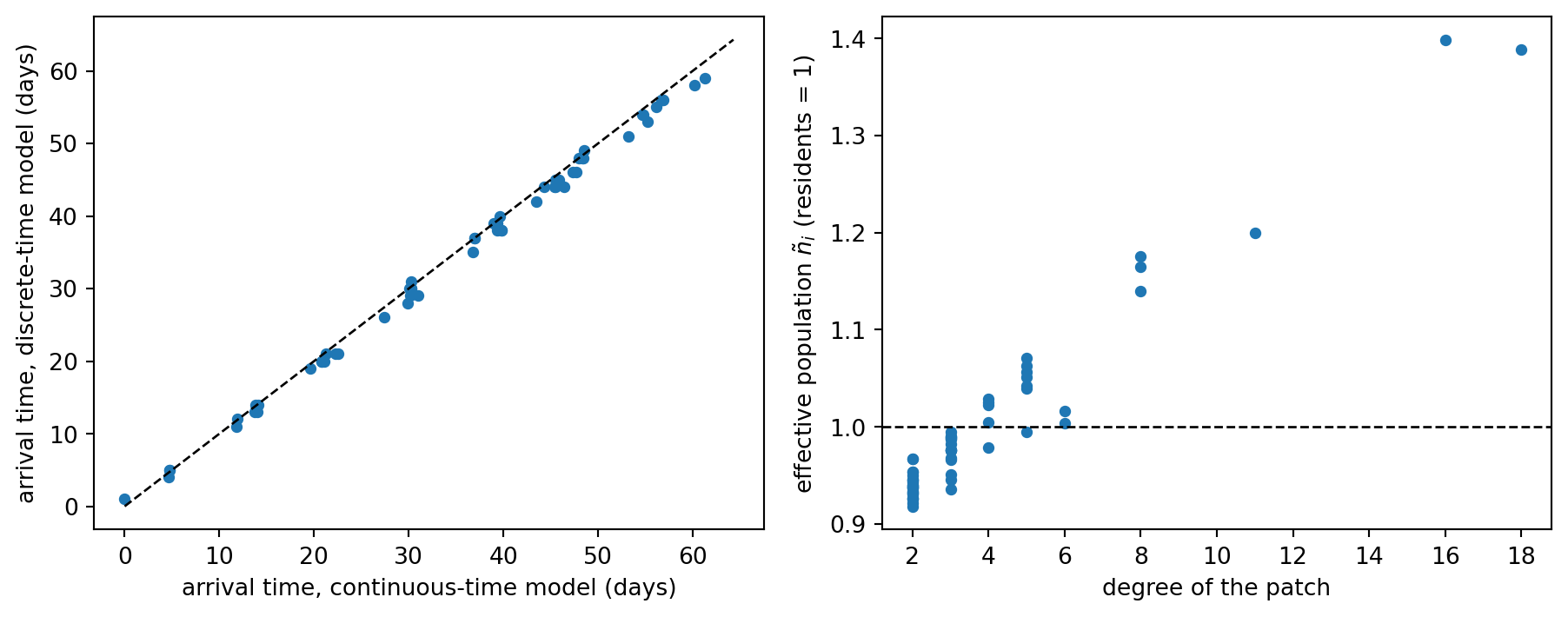
#| fig-cap: "Discrete-time mobility model (reduced from Arenas et al.). Left: arrival time in each patch of the 60-patch small-world graph, discrete-time model with p = 0.1 against the continuous-time model with sigma = 0.01 (same seed, same threshold); the dashed line is the identity. Right: effective population of each patch of the Barabási-Albert graph against its degree: patches with more links receive more commuters than they send."
def simulate_mmca(G, p, beta_c=0.03, k_bar=10, mu=0.1, t_max=300, seed_patch=0, i0=1e-3, thr=1e-4):
    """Reduced Markov-chain metapopulation SIR with equal patch populations (n_j = 1)."""
    n = G.number_of_nodes()
    A = nx.to_numpy_array(G, nodelist=range(n))
    R = A / A.sum(axis=1)[:, None]
    M = (1 - p) * np.eye(n) + p * R              # M[j, i]: fraction of residents of j present in i
    n_eff = M.sum(axis=0)                        # effective populations
    rS, rI, rR = np.ones(n), np.zeros(n), np.zeros(n)
    rS[seed_patch] -= i0
    rI[seed_patch] = i0
    arrival, totals = np.full(n, np.nan), []
    for t in range(1, t_max + 1):
        X = (M.T @ rI) / n_eff
        P = 1 - (1 - beta_c) ** (k_bar * X)
        Pi = (1 - p) * P + p * R @ P
        new = Pi * rS
        rS, rI, rR = rS - new, rI + new - mu * rI, rR + mu * rI
        totals.append(rS + rI + rR)
        arrival[np.isnan(arrival) & (rI > thr)] = t
    return arrival, np.array(totals), n_eff


G_sw = patch_graphs["small-world (p = 0.1)"]
arr_mmca, totals, n_eff = simulate_mmca(G_sw, 0.1)
fig, axes = plt.subplots(1, 2, figsize=(9.5, 3.8))
axes[0].plot(arrival["small-world (p = 0.1)"], arr_mmca, "o", ms=4)
lim = [0, max(np.nanmax(arr_mmca), np.nanmax(arrival["small-world (p = 0.1)"])) + 3]
axes[0].plot(lim, lim, "k--", lw=1)
axes[0].set_xlabel("arrival time, continuous-time model (days)")
axes[0].set_ylabel("arrival time, discrete-time model (days)")

G_ba = patch_graphs["Barabási-Albert (m = 2)"]
_, _, n_eff_ba = simulate_mmca(G_ba, 0.1)
deg_ba = np.array([G_ba.degree(k) for k in range(n_patches)])
axes[1].plot(deg_ba, n_eff_ba, "o", ms=4)
axes[1].axhline(1, color="k", ls="--", lw=1)
axes[1].set_xlabel("degree of the patch")
axes[1].set_ylabel("effective population $\\tilde n_i$ (residents = 1)")
plt.tight_layout()
plt.show()

print(f"sum of effective populations = {n_eff_ba.sum():.6f} (total population = {n_patches}); "
      f"range of n_eff on the BA graph: {n_eff_ba.min():.2f} to {n_eff_ba.max():.2f}")
print(f"max |N_k - 1| over time = {np.abs(totals - 1).max():.1e}")
print(f"Spearman correlation of the two arrival times (small-world graph): "
      f"{spearmanr(arrival['small-world (p = 0.1)'], arr_mmca)[0]:.3f}")
print("patches never reached with p = 0:", int(np.isnan(simulate_mmca(G_sw, 0.0)[0]).sum()), "of", n_patches)
```
Three checks support the implementation. The total population is conserved to rounding error. The effective populations add up to the total population, as they must, but individual patches differ: on the Barabási-Albert graph the busiest patch hosts about 1.4 times its residents at the time of contact. Finally, with $p = 0$ there is no mobility and 59 of the 60 patches are never reached. The arrival times of the discrete-time model agree with those of the continuous-time model on the same graph, although the two parameter sets were chosen only to give similar growth rates and not fitted to each other; what the two share is the mobility network.
## Restricting mobility: what changes and what does not
A restriction of travel reduces $\sigma$ in the continuous model or $p$ in the discrete one. @fig-meta-arrival shows its effect on the arrival time. What it does not change is the epidemic inside each patch. The table reports, for three values of $\sigma$ on the small-world graph, the delay and the final size of the epidemic in the patches, to be compared with the final size relation $z = 1 - e^{-R_0 z}$ of [The Final Size of an Epidemic](../low-dimensional-dynamics/final-size.qmd).
```{python}
from scipy.optimize import brentq

z_th = brentq(lambda z: z - 1 + np.exp(-(beta / gamma) * z), 1e-9, 1.0)
print(f"final size relation for R0 = {beta / gamma:.0f}: z = {z_th:.4f}")
print(f"{'sigma':>8}{'mean arrival':>14}{'delay vs sigma = 0.01':>24}{'mean final size':>17}{'min final size':>16}")
base = np.nanmean(arrival["small-world (p = 0.1)"])
for s in (0.1, 0.01, 0.001):
    arr, sol, _ = simulate_patches(G_sw, s, t_max=1500)
    final = sol.y[2 * n_patches:, -1]
    print(f"{s:>8}{np.nanmean(arr):>14.1f}{np.nanmean(arr) - base:>24.1f}{final.mean():>17.4f}{final.min():>16.4f}")
```
Restricting mobility by a factor of ten delays the arrival by weeks but leaves the final size in each patch at 0.935 to 0.939, within 0.6% of the value 0.9405 of an isolated population with $R_0 = 3$. This is a statement about the model in which each patch has $R_0 > 1$ by itself: mobility only decides when the patches are infected, and only measures that reduce transmission inside the patches (smaller $\beta$) change the final size. @arenas2020modeling derive the effective reproduction number of the whole system as a function of the mobility and confinement parameters, which is the quantity that decides whether an epidemic is suppressed. The statistical analysis of @barbeito2023effectiveness looks at the same question from the data side: an increase of one standard deviation in the overall stringency index over nine fields of activity was associated with a 22% lower growth of the 7-day cumulative incidence over the following week in Spain between September 2020 and May 2021 (relative risk 0.78). Among single fields, culture and leisure and social distancing showed the largest effects, although culture and leisure was no longer significant in a model with fewer fields.
::: {.callout-note}
## Exercise 2: what mobility restrictions cannot do
Explain with the final size relation why restricting mobility on this model cannot reduce the final size, and name the parameter that would. For which value of $R_0$ inside the patches would mobility restrictions determine whether the epidemic occurs?
:::
::: {.callout-tip collapse="true"}
## Solution
Within a patch the final size solves $z = 1 - e^{-R_0 z}$ in the limit of weak coupling, a relation that does not contain $\sigma$. Restricting mobility only postpones the moment at which the patches start their own epidemics. The parameters that change $z$ are those that change $R_0 = \beta/\gamma$, such as contact reduction or vaccination. If $R_0 < 1$ inside every patch, an epidemic in one patch dies out locally and mobility has no influence on whether the epidemic occurs. For $R_0$ slightly above 1, the delay is not the main effect: the epidemic is slow in each patch, and the importation of cases matters for whether it takes off.
:::
## What's Next?
The next module of this document set returns to simulation of agents. For the network material itself, [Practice: Propagation](practice-propagation.qmd) asks you to simulate spreading on a real network; a metapopulation of cities connected by flights is the natural next model, with the US flights network of [Practice: Flights and Other Networks](practice-flights-network.qmd) as the mobility graph.