---
title: "What Nagel and Schreckenberg Did"
subtitle: "Module 6: Explorables and Discrete Models"
format: html
---
::: {.callout-note}
## Reading
- **Compulsory:** @nagel1992cellular, the whole paper (nine pages). Concentrate on Sections 2 to 5 and on Figures 4 to 6.
:::
This page reports what the original paper defines, measures and concludes, and checks each number against our own simulations. Read the paper first and use this page as a guide, not as a substitute. The rules themselves are on the page [The Nagel-Schreckenberg Model](nagel-schreckenberg.qmd).
## The claim of the paper
Nagel and Schreckenberg ask whether a Boolean, fully discrete model can reproduce the transition from laminar traffic to start-stop waves that appears when the vehicle density increases [@nagel1992cellular]. They argue that it can: a stochastic cellular automaton shows this transition, and analytical results are available for special cases. The authors also report that, with an open road and a bottleneck, the simulated system reaches a state of its own accord, and they note a resemblance to self-organised criticality. They leave a quantitative treatment of this state, and of the case $v_{\max} > 1$, to later work.
## The model as the paper defines it
The paper allows open or periodic boundaries. Each vehicle has an integer velocity between $0$ and $v_{\max}$, and one update consists of four steps carried out in parallel [@nagel1992cellular]:
1. *Acceleration.* If $v < v_{\max}$ and the distance to the next car ahead is larger than $v + 1$, then $v \to v + 1$.
2. *Slowing down.* If the next car is at distance $j \le v$ sites, then $v \to j - 1$.
3. *Randomization.* With probability $p$, a car with $v > 0$ reduces its speed by one.
4. *Motion.* Each car advances $v$ sites.
Here "distance" is the difference between site indices, so the number of empty cells in between is the distance minus one. The paper's acceleration step carries the condition on the distance, while the page [The Nagel-Schreckenberg Model](nagel-schreckenberg.qmd) writes $v \leftarrow \min(v+1, v_{\max})$ followed by $v \leftarrow \min(v, d)$ with $d$ the number of empty cells. The two forms give the same new speed. The chunk below confirms this on 20 000 random configurations, with the same random numbers in both versions.
```{python}
import numpy as np
from amlab.cellular_automata.traffic_models import gaps_ahead

L, vmax = 60, 5
rng = np.random.default_rng(0)
agree = True
for _ in range(20_000):
    n = rng.integers(1, 40)
    x = np.sort(rng.choice(L, n, replace=False))
    gap = gaps_ahead(x, L)
    v = np.minimum(rng.integers(0, vmax + 1, n), gap)      # a legal state
    rand = rng.random(n) < 0.4                              # shared random draws
    dist = gap + 1                                          # paper: difference of site indices
    v_paper = np.where((v < vmax) & (dist > v + 1), v + 1, v)
    v_paper = np.minimum(v_paper, dist - 1)
    v_paper = np.where(rand & (v_paper > 0), v_paper - 1, v_paper)
    v_page = np.minimum(np.minimum(v + 1, vmax), gap)
    v_page = np.where(rand & (v_page > 0), v_page - 1, v_page)
    agree &= np.array_equal(v_paper, v_page)
print("The two formulations agree:", agree)
```
The paper stresses that step 3 is essential. Without it the dynamics is deterministic, and every initial configuration quickly reaches a stationary pattern that moves backwards, against the traffic, by one site per time step [@nagel1992cellular]. In our simulations of the jammed regime ($\rho > 1/(v_{\max}+1)$, $p = 0$, $v_{\max}=5$), the occupancy pattern was shifted by exactly one site to the left in every step, for $\rho = 0.3$, $0.4$ and $0.5$. This statement therefore holds in the congested phase. In free flow ($\rho < 1/(v_{\max}+1)$) the stationary pattern moves forward with the cars instead.
## How the paper measures the flow
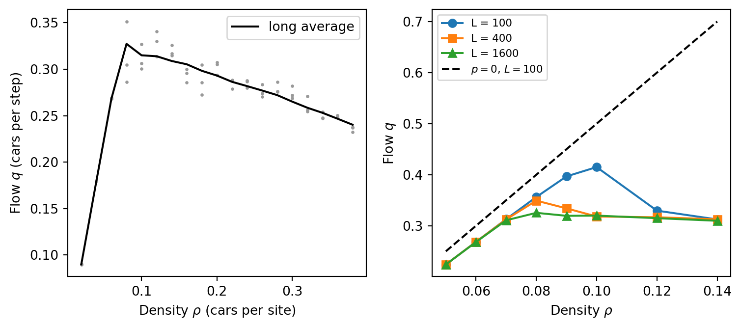
The paper measures the flow in the way a road detector does. It starts from random positions with all speeds equal to zero, discards the first $t_0 = 10 L$ steps, and then records the time-averaged occupancy and the time-averaged number of cars that pass a fixed pair of neighbouring sites [@nagel1992cellular]. For a ring of $L$ cells the flow measured at a fixed site equals $\sum_n v_n / L$ on average, which is the definition on the page [The Fundamental Diagram](fundamental-diagram.qmd). Figure 4 of the paper uses $L = 10^4$. Its dots are averages over 100 steps and can be compared with real detector data (Figure 5), and its line is an average over $10^6$ steps.
::: {.callout-note}
## Which value of $p$?
The captions and the text I read do not state the value of $p$ for Figures 4 and 6. Two details point to $p = 0.5$: the paper calls $4.5$ sites per step the mean speed in free traffic, which equals $v_{\max} - p$ for $v_{\max} = 5$ (see the scale argument below), and the data-file label printed inside Figure 6 reads `V5/p.5/...`. Our simulations at $p = 0.5$ reproduce the numbers quoted in the paper, which supports this reading. The value of $p$ is nevertheless inferred, not quoted.
:::
```{python}
#| echo: false
#| label: fig-paper-fd
#| fig-cap: 'Reproduction of the closed-system experiment of the paper (v_max = 5, p = 0.5, random start at rest, burn-in 10 L steps, ring of 1000 cells). Left: flow against density. Dots are averages over 100 steps, three per density, and the line is the average over 20 000 steps. Right: flow near the maximum for rings of 100, 400 and 1600 cells, and for p = 0 (dashed) on the ring of 100 cells. The maximum depends on the system size for p = 0.5 but not for p = 0.'
#| fig-width: 8
#| fig-height: 3.6
import numpy as np
import matplotlib.pyplot as plt
from amlab.cellular_automata.traffic_models import nasch_step, ring_initial
def flow_series(length, rho, p, steps, burn_in, vmax=5, seed=0):
"""Instantaneous flow sum(v)/L for every step after the burn-in."""
rng = np.random.default_rng(seed)
x, v = ring_initial(length, int(round(rho * length)), "random", vmax, rng)
out = np.empty(steps - burn_in)
for t in range(steps):
x, v = nasch_step(x, v, length, vmax, p, None, rng)
if t >= burn_in:
out[t - burn_in] = v.sum() / length
return out
L = 1000
dens = np.round(np.arange(0.02, 0.40, 0.02), 3)
line, dots = [], []
for i, rho in enumerate(dens):
s = flow_series(L, rho, 0.5, burn_in=10 * L, steps=10 * L + 20_000, seed=i)
line.append(s.mean())
dots.append([s[a:a + 100].mean() for a in (0, 7000, 14000)])
fig, (ax1, ax2) = plt.subplots(1, 2, figsize=(8, 3.6))
for rho, d in zip(dens, dots):
ax1.plot([rho] * len(d), d, ".", color="0.6", markersize=3)
ax1.plot(dens, line, "k-", label="long average")
ax1.set_xlabel(r"Density $\rho$ (cars per site)")
ax1.set_ylabel(r"Flow $q$ (cars per step)")
ax1.legend(loc="upper right")
zoom = np.array([0.05, 0.06, 0.07, 0.08, 0.09, 0.10, 0.12, 0.14])
for length, mk in ((100, "o"), (400, "s"), (1600, "^")):
q = [flow_series(length, r, 0.5, 10 * length + 10_000, 10 * length, seed=3).mean() for r in zoom]
ax2.plot(zoom, q, marker=mk, label=f"L = {length}")
q0 = [flow_series(100, r, 0.0, 3000, 1000, seed=3).mean() for r in zoom]
ax2.plot(zoom, q0, "k--", label=r"$p=0$, $L=100$")
ax2.set_xlabel(r"Density $\rho$")
ax2.set_ylabel(r"Flow $q$")
ax2.legend(fontsize=8)
plt.tight_layout()
plt.show()
```
The paper reports that the change from laminar to jammed flow takes place near $\rho \approx 0.08$, that the position and shape of the maximum of $q(\rho)$ depend on the system size when $p > 0$, and that simulations without randomization show no such dependence [@nagel1992cellular]. It adds that it is not clear from the plots where an exact transition point lies. Our simulations show the same three features. For $p = 0.5$ the maximum is at $\rho \approx 0.08$ to $0.10$ with $q \approx 0.32$ on large rings (a ring of $10^4$ cells, checked separately, gives $q = 0.316$, $0.321$ and $0.321$ at $\rho = 0.08$, $0.09$ and $0.10$), the right panel of @fig-paper-fd shows a higher maximum on short rings, and the $p = 0$ curve does not move.
## The exactly solvable case $v_{\max} = 1$
For $v_{\max} = 1$ the acceleration step is trivial, because every car reaches speed 1 in one step, so each car only asks whether the next site is free and whether it is randomly stopped. The paper treats random sequential update in continuous time, where a car at site $i$ jumps to $i + 1$ at rate $1 - p$ if that site is free [@nagel1992cellular]. In that case the factor $1-p$ only rescales time, all values of $p < 1$ share the same stationary distribution, every configuration with a given number of cars is equally likely, and the flow is
$$
q(\rho) = \rho\,(1 - \rho),
$$ {#eq-nasch-rs-flow}
the probability that a car has a free site in front of it (Equation 7 of the paper). The paper adds that the parallel update gives a different function that is also symmetric about $\rho = 1/2$.
The chunk below checks both statements numerically. The random sequential update is run with hop probability $1 - p$ per attempt, so that the measured flow in hops per site per sweep is $(1-p)\rho(1-\rho)$, which is @eq-nasch-rs-flow with the time axis rescaled by $1-p$. The parallel update is run with the course code, and the parallel flow at $\rho$ and $1 - \rho$ is compared.
```{python}
import numpy as np
from amlab.cellular_automata.traffic_models import mean_flow


def random_sequential_flow(rho, p, length=400, sweeps=1500, burn_in=300, seed=0):
    rng = np.random.default_rng(seed)
    occ = np.zeros(length, dtype=bool)
    occ[rng.choice(length, int(round(rho * length)), replace=False)] = True
    hops = 0
    for s in range(sweeps):
        for i in rng.integers(0, length, length):
            j = (i + 1) % length
            if occ[i] and not occ[j] and rng.random() < 1 - p:
                occ[i], occ[j] = False, True
                hops += s >= burn_in
    return hops / (length * (sweeps - burn_in))


p = 0.5
for rho in (0.2, 0.5):
    print(f"random sequential, rho = {rho}: q = {random_sequential_flow(rho, p):.3f},"
          f"  (1-p) rho (1-rho) = {(1 - p) * rho * (1 - rho):.3f}")

for rho in (0.2, 0.3, 0.4):
    q1 = mean_flow(2000, int(rho * 2000), 6000, 2000, vmax=1, p=p, seed=2)
    q2 = mean_flow(2000, int((1 - rho) * 2000), 6000, 2000, vmax=1, p=p, seed=2)
    print(f"parallel update, v_max = 1: q({rho}) = {q1:.3f}, q({1 - rho:.1f}) = {q2:.3f}")
```
The run gave $q = 0.080$ and $0.127$ for the random sequential update, against the predictions $0.080$ and $0.125$, and equal flows at $\rho$ and $1-\rho$ for the parallel update, up to sampling noise of about 0.002 (for example $0.119$ at $\rho = 0.3$ and $0.7$).
## The open road with a bottleneck
In Section 4 the paper changes only the boundaries. A car with speed $0$ is placed on the first site whenever that site is empty, which models a saturated wider road that feeds a single lane, and every car that reaches the last six sites is deleted [@nagel1992cellular]. After relaxation the paper reports a density $\langle\rho_c\rangle = 0.069 \pm 0.002$ and a flow $\langle q_c\rangle = 0.304 \pm 0.001$, from rings of up to $10^4$ sites and runs of up to $5 \times 10^6$ steps. Figure 6 shows that this self-organised state lies at a lower flow than the maximum of the closed system for $v_{\max} = 5$, while for $v_{\max} = 1$ the open system drives itself to the maximum flow at $\rho = 1/2$.
The paper does not say in which order the update and the boundary operations are applied. The code below applies them after the update, which is one reasonable choice.
```{python}
import numpy as np


def bottleneck(length=2000, steps=150_000, burn_in=30_000, vmax=5, p=0.5, seed=0):
    """Open road: inject a car with v = 0 when cell 0 is empty, delete cars in the last 6 cells."""
    rng = np.random.default_rng(seed)
    x = np.array([], dtype=int)
    v = np.array([], dtype=int)
    left, right = length // 4, 3 * length // 4        # measure the density in the middle half
    n_out, occupied, n_obs = 0, 0.0, 0
    for t in range(steps):
        if x.size == 0 or x[0] > 0:
            x = np.concatenate(([0], x))
            v = np.concatenate(([0], v))
        gap = np.append(np.diff(x) - 1, 10**6)         # the front car sees a free road
        v = np.minimum(np.minimum(v + 1, vmax), gap)
        v = np.where(rng.random(x.size) < p, np.maximum(v - 1, 0), v)
        x = x + v
        gone = x >= length - 6
        if t >= burn_in:
            n_out += gone.sum()
            occupied += ((x >= left) & (x < right)).sum() / (right - left)
            n_obs += 1
        x, v = x[~gone], v[~gone]
    return occupied / n_obs, n_out / (steps - burn_in)


rho_c, q_c = bottleneck()
print(f"density {rho_c:.3f}, flow {q_c:.3f}")
```
The chunk gives a density of $0.069$ and a flow of about $0.306$. Two longer runs with different seeds ($3 \times 10^5$ steps on the same ring of 2000 sites) gave densities $0.0688$ and $0.0685$ and flows $0.3041$ and $0.3042$. All of these agree with the values of the paper, which are $0.069 \pm 0.002$ and $0.304 \pm 0.001$. For comparison, the closed ring at $p = 0.5$ reaches $q \approx 0.32$ at its maximum (previous section), so the bottleneck state indeed lies below the maximum flow.
## The scale argument and the comparison with real traffic
Section 5 fixes the units in four ways and finds that they agree in order of magnitude [@nagel1992cellular].
1. *Length and mean speed.* A car occupies about 7.5 m in a complete jam, so one site is 7.5 m. Free traffic with $4.5$ sites per step should correspond to about 120 km/h, which gives a time step of about 1 s.
2. *Position of the maximum.* Real measurements put the maximum of the flow at about 30 vehicles per kilometre and lane, which is $0.225$ vehicles per 7.5 m. This is about twice the position of the maximum in the simulation.
3. *Capacity.* A freeway lane carries about 2000 vehicles per hour, which is $0.56$ vehicles per second. The simulated maximum of $0.32$ vehicles per step then suggests a time step of about $0.5$ s.
4. *Speed of the backward wave.* Start-stop waves travel backwards at about 15 km/h, or 4.2 m/s. With a maximum capacity of about $0.3$ cars per step, the paper takes $0.3$ sites, that is $2.25$ m, per step as the speed of the backward wave.
The paper concludes that the parameters of a discrete model are rather rigid once one accepts one car per site in a jam. The comparison is deliberately rough. Figure 5 shows measured flow in vehicles per hour against occupancy in per cent. The caption gives the units of occupancy as "cars per hour", which is evidently a misprint.
::: {.callout-note}
## Exercise
Redo the four scale estimates with the numbers quoted in the paper. Which of them reproduces the value that the paper prints?
:::
::: {.callout-tip collapse="true"}
## Solution
(1) $7.5 \times 4.5 / (120/3.6) = 33.75 / 33.3 = 1.01$ s. (2) The position of the maximum is not a time estimate. $0.225 / 0.08 \approx 2.8$, so the model maximum is lower in density by a factor of 2 to 3, which the paper rounds to "about 2". (3) $0.32 / 0.56 = 0.57$ s, printed as about 0.5 s. (4) $2.25 / 4.2 = 0.54$ s, whereas the paper prints "about 0.7 seconds" and describes it as lying between the first and the third estimate. The ratio is 0.54 s, which is almost the same as the third estimate, so the printed value is not consistent with the quoted inputs. The conclusion that a time step corresponds to roughly one second, within a factor of two, is not affected. Check also that $135$ km/h for $v_{\max} = 5$ and $7.5$ m per cell is the speed of a car at the maximum speed, whereas the paper's 120 km/h refers to the mean speed $v_{\max} - p = 4.5$.
:::
## Queueing picture of a jam
At the end of Section 5 the paper offers a remark that goes beyond the numbers [@nagel1992cellular]. A jam of a given length gains a car at its rear with some probability per step and loses one at its front with another probability per step. Because the departure rate of one jam fixes the arrival rate at the next, all clusters behave like queues at the critical point where the two rates coincide. The authors suggest that start-stop waves may be a queueing phenomenon in which only the formation of the jam is dynamical. This is a conjecture of the paper. It is not tested there.
::: {.callout-note}
## Exercise
Measure the back-travelling speed of the jams in your own simulation for $v_{\max} = 5$ and $p = 0.5$ on a ring of 2000 cells at $\rho = 0.2$, $0.3$ and $0.4$. Record the positions of the cars with $v = 0$ at every step, correlate the pattern at time $t$ with that at $t + 20$ for shifts between $-60$ and $+10$ cells, and take the shift with the largest correlation divided by $20$. Compare with the number $0.3$ that the paper uses.
:::
::: {.callout-tip collapse="true"}
## Solution
Our measurement, with the pattern of stopped cars correlated over a lag of 20 steps and two seeds, gave $-0.35$ to $-0.40$ sites per step, with the same value for both seeds at each density. The magnitude is close to the $0.3$ used in the paper, but the paper's value is an estimate from the maximum capacity, not a measurement of jams. The two numbers need not coincide, and with the lag, grid and averaging we used, the measured speed has a resolution of about $0.05$ sites per step. The page [From Cars to a Continuum](traffic-continuum.qmd) compares the jam speed with the slope of the fundamental diagram.
:::
## What the paper does not do
- It does not fit $p$ or $v_{\max}$ to data. It argues that $v_{\max} = 5$ is the realistic choice "for reasons stated below", and then fixes the scales.
- It does not locate the transition point. It states that the position and form of the maximum depend on the system size.
- It states the result for $v_{\max} > 1$ in terms of a mean-field treatment to be reported elsewhere, and its Reference 12 is announced as "in preparation".
- It does not investigate lane changes. They are announced as a topic for later investigations. The page [Traffic Extensions](traffic-extensions.qmd) gives some of the later work.