Gierer-Meinhardt Solver in 2D
Module 4: Space and Pattern Formation
The reaction terms are those of the 1D laboratory (Gierer and Meinhardt 1972). Only the Laplacian and the array shape change:
\[ \begin{aligned} \frac{\partial u}{\partial t} &= \Delta u + \gamma \left(a - b u + \frac{u^2}{v}\right), \\ \frac{\partial v}{\partial t} &= d\,\Delta v + \gamma \left(u^2 - v\right), \end{aligned} \tag{1}\]
with \(u\) and \(v\) now functions of \((x, y, t)\).
Core activity
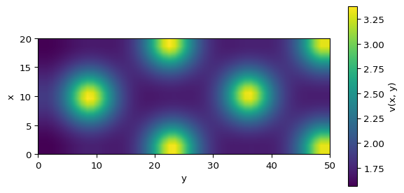
Simulate Case A (\(a = 0.4\), \(b = 1\), \(d = 30\), \(\gamma = 1\)) and Case B (\(d = 20\)) on the rectangle \(L_x = 20\), \(L_y = 50\) with Neumann boundaries, and compare with the mode predictions on Unstable Modes in 2D.
Initialize the Grid
Exercise
Create the perturbed steady state on the rectangle.
import numpy as np

rng = np.random.default_rng(3)

length_x, length_y, dx = 20, 50, 1.0
num_x = int(length_x / dx)
num_y = int(length_y / dx)
u_star = 1.4  # (a + 1) / b for a = 0.4, b = 1

# TODO: create the homogeneous state (u_star, u_star**2), shape (2, num_x, num_y)
uv =

# TODO: add 1% multiplicative noise
uv =
Solution
uv = np.array([u_star, u_star**2])[:, None, None] * np.ones((2, num_x, num_y))
uv = uv * (1 + 0.01 * rng.standard_normal((2, num_x, num_y)))
Build the PDE Right-Hand Side
Exercise
Reuse laplacian_2d for both species and add the reaction terms.
def gierer_meinhardt_pde_2d(t, uv, gamma=1, a=0.40, b=1.00, d=30, dx=1.0):
    u, v = uv
    lu = laplacian_2d(u, dx)
    lv = laplacian_2d(v, dx)

    # TODO: write the reaction terms and combine them with diffusion
    du_dt =
    dv_dt =
    return np.array([du_dt, dv_dt])
Solution
def gierer_meinhardt_pde_2d(t, uv, gamma=1, a=0.40, b=1.00, d=30, dx=1.0):
    u, v = uv
    lu = laplacian_2d(u, dx)
    lv = laplacian_2d(v, dx)

    f = a - b * u + (u**2) / v
    g = u**2 - v
    du_dt = lu + gamma * f
    dv_dt = d * lv + gamma * g
    return np.array([du_dt, dv_dt])
Time Step with Euler’s Method
Once the right-hand side is available, the full update is explicit Euler applied to the whole array,
\[ UV^{n+1} = UV^n + dt\,G(UV^n), \]
followed by one boundary update. The order matters. First compute the Euler step, then reapply the edge values, so the next stencil evaluation sees data consistent with the boundary condition. Validate with a long loop and one snapshot before you animate.
Exercise
Complete the loop: one vectorized Euler update, then one boundary update.
dt = 0.005          # below the 2D bound dx**2 / (4 d) = 0.0083
num_iter = 80000    # t = 400

for _ in range(num_iter):
    # TODO: Euler update of uv
    # TODO: reapply Neumann boundary conditions
    pass
Solution
for _ in range(num_iter):
    uv = uv + dt * gierer_meinhardt_pde_2d(0, uv, d=30, dx=dx)
    uv = apply_boundary_conditions(uv, bc="neumann")
Validation
- Time step. In 2D the bound is \(dt \le dx^2/(4d)\). Check it before every new grid (Time-Step Stability).
- Convergence. Rerun with \(dx = 0.5\) and \(dt\) divided by four on a smaller domain and check that the spacing of the spots does not change.
- Prediction. Case B should return to the flat state. Case A should form a pattern whose spacing matches the unstable modes.
Case A forms spots. Unstable Modes in 2D compares this with the list of unstable modes.
Tip
Reference code is available in amlab/pdes_2d/gierer_meinhardt_2d.py.
References
Gierer, Alfred, and Hans Meinhardt. 1972. “A Theory of Biological Pattern Formation.” Kybernetik 12 (1): 30–39. https://doi.org/10.1007/BF00289234.