---
title: "Scaling of Path Length and Clustering"
subtitle: "Module 5: Complex Networks"
format: html
---
::: {.callout-note}
## Reading
- **Compulsory:** @watts1998collective, the first two pages (definition of $L(p)$ and $C(p)$, and the regime $n \gg k \gg \ln n \gg 1$).
- **Recommended:** @newman2003structure, Section 3.1 (small-world effect), Section 4.1 (random graph), Section 6 (small-world model) and Section 7.2 (Barabási-Albert model).
:::
Each model is summarised by three columns: the average path length $L$, the clustering $C$ and the degree distribution $p(k)$. Entries such as "$L \sim \log N$" or "$C \approx \langle k \rangle / N$" are statements about how a quantity **changes with the size $N$** of the network. A single graph cannot confirm them. This page measures $L$ and $C$ for graphs of increasing size, compares the measurements with the formulas of the lecture, and states where the formulas hold only asymptotically.
## Definitions
For a connected graph with $N$ nodes the average path length is
$$
L = \frac{1}{N(N-1)} \sum_{i \neq j} d(i,j),
$$ {#eq-L}
where $d(i,j)$ is the length of the shortest path between $i$ and $j$. A network is called **small-world** if $L$ grows like $\log N$ or more slowly. The average clustering is $C = \frac{1}{N}\sum_i C_i$ with $C_i = 2E_i/\big(k_i(k_i-1)\big)$, where $E_i$ is the number of edges among the neighbours of node $i$ [@watts1998collective]. A real network is considered clustered when $C \gg C_{\text{random}}$, the value of a random graph with the same $N$ and $\langle k \rangle$.
## Theoretical predictions
| Model | $L$ | $C$ | Source of the formula |
|---|---|---|---|
| Erdős-Rényi | $\ln N / \ln \langle k \rangle$ | $\langle k \rangle / N$ | $\langle k \rangle^{\ell} \sim N$; $C = p$ |
| Watts-Strogatz, $p = 0$ | $\approx N / (2k)$ | $3(k-2) / \big(4(k-1)\big)$ | ring lattice |
| Watts-Strogatz, $p > 0$ | $\sim \ln N$ for $N$ large enough | $\approx C(0)\,(1-p)^3$ | shortcuts; see [Small-World Networks](small-world.qmd) |
| Barabási-Albert | smaller than ER | decreases with $N$ | hubs |
The Erdős-Rényi estimate follows from counting: the number of nodes at distance $\ell$ from a given node grows like $\langle k \rangle^{\ell}$, so the whole graph is reached when $\langle k \rangle^{\ell} \sim N$ [@newman2003structure, Section 4.1]. For the ring lattice, @watts1998collective give $L \approx n/2k$ and $C \to 3/4$ as $k$ grows. In the Watts-Strogatz entry $k$ is the full degree of the ring lattice, as in `nx.watts_strogatz_graph`.
## Measurement
Computing $L$ exactly needs a shortest-path search from every node. The helper below averages the distances from at most 300 randomly chosen source nodes, which is exact for $N \le 300$ and, in a test at $N = 3200$ with five different source samples, deviated from the exact value by at most 1.5%. It works on the largest connected component. All graphs have mean degree 6 ($k = 6$ for Watts-Strogatz, $m = 3$ for Barabási-Albert and for the clustered variant introduced in [Triadic Closure](triadic-closure.qmd)). Each point is an average over 3 graphs.
```{python}
import matplotlib.pyplot as plt
import networkx as nx
import numpy as np
from scipy.sparse.csgraph import shortest_path

SEED = 7


def avg_path_length(G, n_src=300, seed=0):
    """Average distance in the largest component, from at most n_src random sources."""
    H = G.subgraph(max(nx.connected_components(G), key=len))
    nodes = list(H)
    A = nx.to_scipy_sparse_array(H, nodelist=nodes, format="csr")
    # SciPy's csgraph routines require int32 CSR index buffers in this environment.
    A.indices = A.indices.astype(np.int32)
    A.indptr = A.indptr.astype(np.int32)
    n = len(nodes)
    rng = np.random.default_rng(seed)
    src = np.arange(n, dtype=np.int32) if n <= n_src else rng.choice(n, n_src, replace=False).astype(np.int32)
    D = shortest_path(A, unweighted=True, indices=src)
    return D.sum() / (len(src) * (n - 1))


generators = {
    "ER": lambda N, s: nx.fast_gnp_random_graph(N, 6 / (N - 1), seed=s),
    "WS p=1": lambda N, s: nx.watts_strogatz_graph(N, 6, 1.0, seed=s),
    "WS p=0.1": lambda N, s: nx.watts_strogatz_graph(N, 6, 0.1, seed=s),
    "WS p=0.01": lambda N, s: nx.watts_strogatz_graph(N, 6, 0.01, seed=s),
    "WS p=0": lambda N, s: nx.watts_strogatz_graph(N, 6, 0.0, seed=s),
    "BA": lambda N, s: nx.barabasi_albert_graph(N, 3, seed=s),
    "HK": lambda N, s: nx.powerlaw_cluster_graph(N, 3, 0.5, seed=s),
}
Ns = np.array([100, 200, 400, 800, 1600, 3200, 6400])
L = {name: [] for name in generators}
C = {name: [] for name in generators}
for name, gen in generators.items():
    for N in Ns:
        graphs = [gen(int(N), SEED + r) for r in range(3)]
        L[name].append(np.mean([avg_path_length(G, seed=r) for r, G in enumerate(graphs)]))
        C[name].append(np.mean([nx.average_clustering(G) for G in graphs]))
    L[name], C[name] = np.array(L[name]), np.array(C[name])
print("done:", list(generators))
```
## Path length
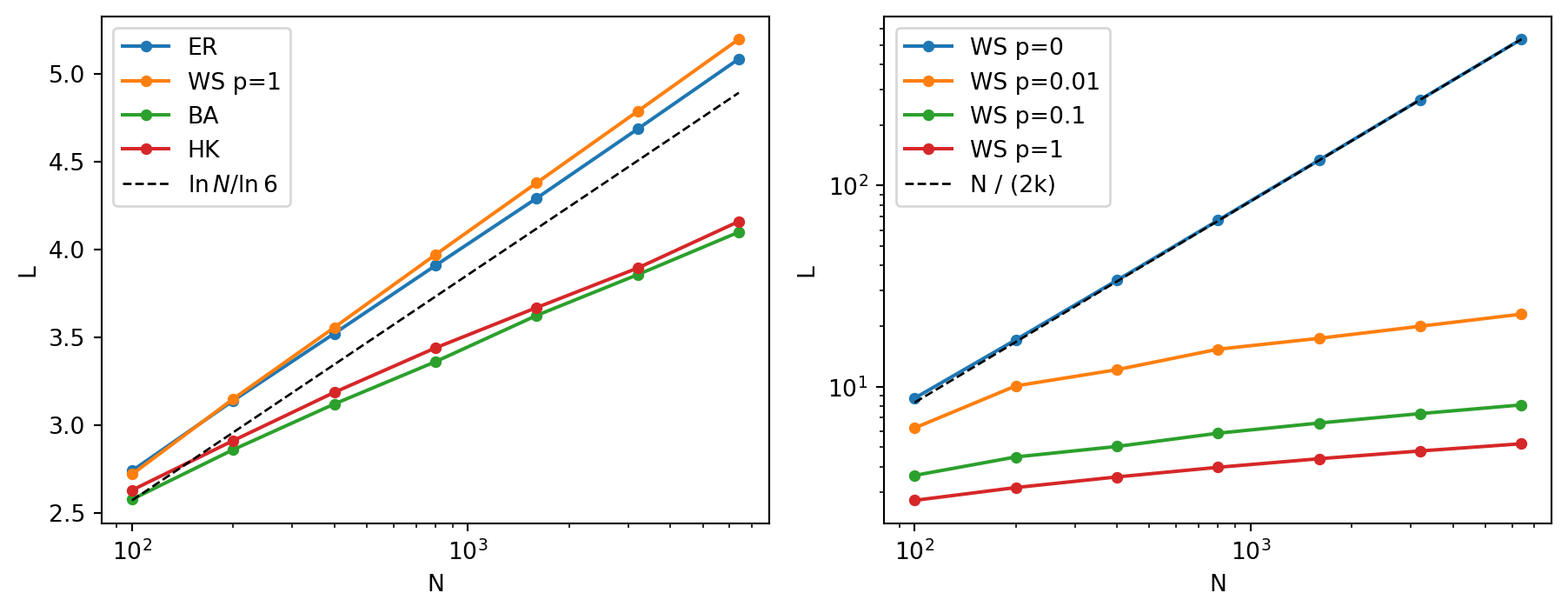
@fig-scaling-L shows the results. In the left panel the models with short paths are compared with the Erdős-Rényi formula; the right panel shows the Watts-Strogatz family from the lattice ($p = 0$) to the random graph ($p = 1$).
```{python}
#| label: fig-scaling-L
#| fig-cap: "Average path length L against the number of nodes N (logarithmic axis), mean degree 6, averages over 3 graphs. Left: Erdős-Rényi (ER), Watts-Strogatz with p = 1 (WS), Barabási-Albert (BA) and the clustered Barabási-Albert variant (HK), with the formula ln N / ln 6 (dashed). Right: Watts-Strogatz for p = 0, 0.01, 0.1 and 1 with the lattice formula N/(2k) (dashed)."
fig, axes = plt.subplots(1, 2, figsize=(9.5, 3.8))
for name in ["ER", "WS p=1", "BA", "HK"]:
    axes[0].semilogx(Ns, L[name], "o-", ms=4, label=name)
axes[0].semilogx(Ns, np.log(Ns) / np.log(6), "k--", lw=1, label=r"$\ln N / \ln 6$")
axes[0].set_xlabel("N")
axes[0].set_ylabel("L")
axes[0].legend()

for name in ["WS p=0", "WS p=0.01", "WS p=0.1", "WS p=1"]:
    axes[1].loglog(Ns, L[name], "o-", ms=4, label=name)
axes[1].loglog(Ns, Ns / 12, "k--", lw=1, label="N / (2k)")
axes[1].set_xlabel("N")
axes[1].set_ylabel("L")
axes[1].legend()
plt.tight_layout()
plt.show()

doubling = lambda y: np.mean(np.diff(y)[2:])   # mean increase of L per doubling of N, N >= 400
print("mean increase of L per doubling of N (N >= 400):")
for name in ["ER", "WS p=1", "WS p=0.1", "BA", "HK"]:
    print(f"  {name:>8}: {doubling(L[name]):.2f}")
print(f"  ln 2 / ln 6 = {np.log(2) / np.log(6):.2f} (ER formula)")
print("L - ln N / ln 6 for ER:", np.round(L["ER"] - np.log(Ns) / np.log(6), 2))
```
Four observations:
- **Erdős-Rényi.** $L$ grows linearly in $\ln N$ with the slope $1/\ln\langle k \rangle$ predicted by the formula. The formula underestimates $L$ by a nearly constant amount of about 0.2: it is a leading-order result.
- **Watts-Strogatz, $p = 1$.** The same logarithmic growth, with practically the same values as Erdős-Rényi: the rewired graph is close to a random graph.
- **Watts-Strogatz, small $p$.** The lattice has $L \approx N/(2k)$. For $p > 0$ the curves leave the lattice line: the shortcuts act as soon as $N$ is large enough for a typical ring to contain some of them. The logarithmic law is a statement about **large** $N$ at fixed $p$. For $p = 0.01$ the curve still grows much faster than a logarithm up to $N = 6400$, and for $p = 0.1$ it approaches the logarithmic slope only slowly. Do not read "$L \sim \log N$" in the Watts-Strogatz row as valid at every size.
- **Barabási-Albert.** At the same mean degree the paths of the scale-free graphs grow more slowly with $N$ than those of the random graph, in line with the statement that for power-law degree distributions $L$ grows no faster than $\ln N / \ln \ln N$ [@newman2003structure, Section 3.1]. The hubs act as shortcuts. The range of $N$ available here is too narrow to distinguish $\ln N/\ln\ln N$ from other slowly growing forms.
## Clustering
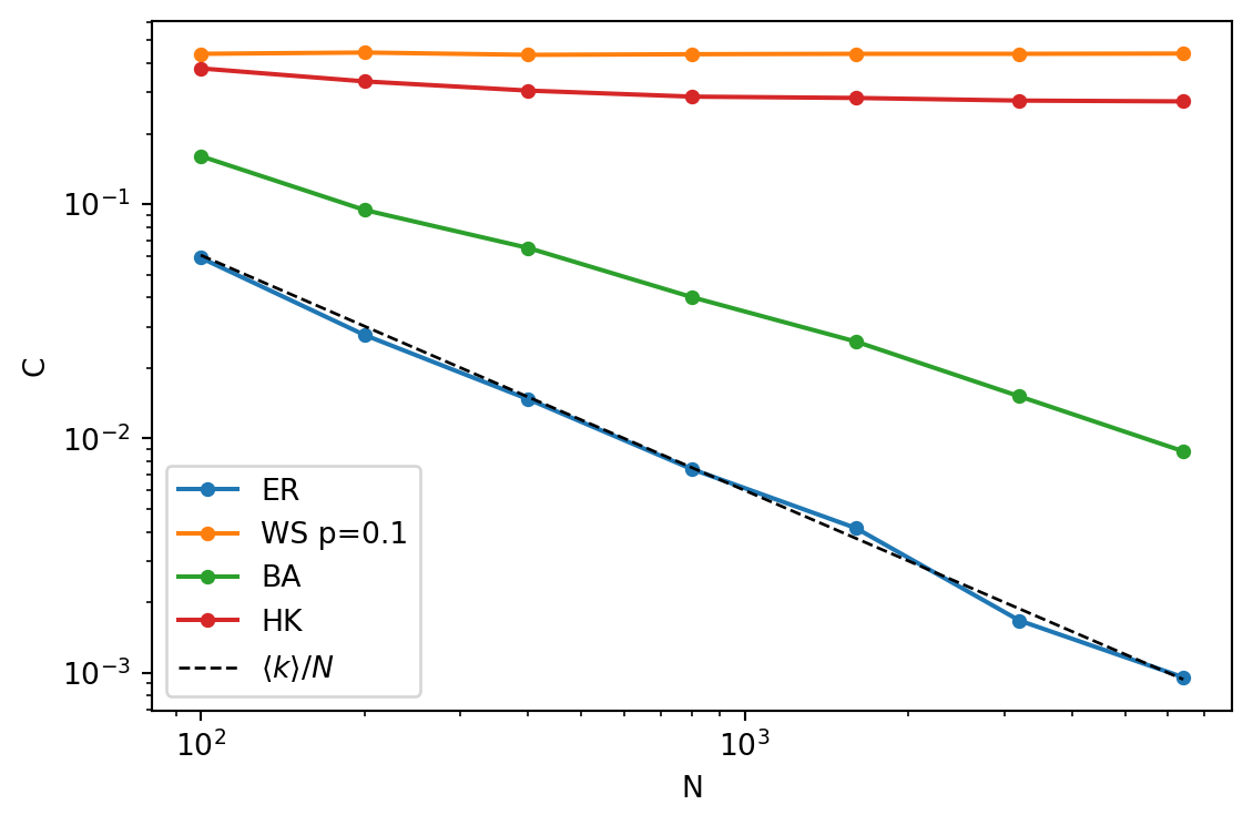
@fig-scaling-C shows $C$ against $N$ on logarithmic axes. A power law $C \propto N^{-\delta}$ is a straight line of slope $-\delta$.
```{python}
#| label: fig-scaling-C
#| fig-cap: "Average clustering coefficient C against N on logarithmic axes, mean degree 6. Erdős-Rényi follows <k>/N (dashed, slope -1). Watts-Strogatz with p = 0.1 and the clustered Barabási-Albert variant (HK) stay at a finite value. The plain Barabási-Albert graph decreases, but more slowly than Erdős-Rényi."
fig, ax = plt.subplots(figsize=(6, 4))
for name in ["ER", "WS p=0.1", "BA", "HK"]:
    ax.loglog(Ns, C[name], "o-", ms=4, label=name)
ax.loglog(Ns, 6 / (Ns - 1), "k--", lw=1, label=r"$\langle k \rangle / N$")
ax.set_xlabel("N")
ax.set_ylabel("C")
ax.legend()
plt.tight_layout()
plt.show()

print("fitted exponent delta in C ~ N^(-delta), N >= 400:")
for name in ["ER", "BA", "WS p=0.1", "HK"]:
    delta = -np.polyfit(np.log(Ns[2:]), np.log(C[name][2:]), 1)[0]
    print(f"  {name:>8}: delta = {delta:.2f}")
print("C(N = 6400): ", {name: round(float(C[name][-1]), 4) for name in ["ER", "BA", "WS p=0.1", "HK"]})
```
The Erdős-Rényi clustering follows $\langle k \rangle / N$ and goes to zero like $1/N$ (fitted exponent close to 1). The Watts-Strogatz graph keeps a finite clustering for any $N$: the rewiring probability fixes the fraction of triangles destroyed, not the size of the graph. The plain Barabási-Albert graph has a clustering that decreases with $N$, with a fitted exponent between that of the random graph and zero; this is a numerical estimate in the range of sizes shown, not a theoretical exponent. The clustered variant of [Triadic Closure](triadic-closure.qmd) stays close to a constant (fitted exponent 0.04, value about 0.27 at $N = 6400$), which is the property that the plain model lacks.
::: {.callout-note}
## Exercise
Use the formula $L \approx \ln N / \ln\langle k \rangle$ to estimate how many nodes an Erdős-Rényi graph with $\langle k \rangle = 6$ needs to have $L = 6$, and compare it with the size you would expect from the measured offset of about 0.2. Then predict from @fig-scaling-L the value of $L$ for a Barabási-Albert graph with $m = 3$ and $N = 10^6$, and say how reliable that extrapolation is.
:::
::: {.callout-tip collapse="true"}
## Solution
From $\ln N = 6 \ln 6$ we get $N = 6^6 \approx 4.7 \times 10^4$. Including the offset, $L = 6$ is reached when $\ln N / \ln 6 + 0.2 = 6$, which gives $N = 6^{5.8} \approx 3.3 \times 10^4$, about 30% fewer nodes, so the leading-order formula is accurate only to within a factor of order one. For Barabási-Albert, extend the measured growth of about 0.25 per doubling of $N$ from $N = 6400$ ($L \approx 4.1$): $\log_2(10^6 / 6400) \approx 7.3$ doublings give $L \approx 6$. This is an extrapolation of a fit over one decade and a half in $N$, and the true functional form is slower than linear in $\ln N$, so treat it as an upper estimate of the order of magnitude, not as a prediction.
:::
::: {.callout-note}
## Exercise
Why is the clustering coefficient of the Watts-Strogatz graph independent of $N$ while that of the Erdős-Rényi graph is not? Answer in terms of the number of triangles per node.
:::
::: {.callout-tip collapse="true"}
## Solution
In the ring lattice each node has exactly $3k(k-2)/8$ triangles around it (9 for $k = 6$), a number that depends only on $k$. Rewiring a fraction $p$ of the edges destroys a fraction of these triangles that depends only on $p$, so $C$ does not depend on $N$. In the Erdős-Rényi graph a node of degree $\langle k \rangle$ has about $\langle k \rangle^2/2$ pairs of neighbours, and each pair is connected with probability $p = \langle k \rangle / N$, so the expected number of triangles per node is about $\langle k \rangle^3/(2N)$, which goes to zero as $N$ grows.
:::
## What's Next?
The next page adds the one ingredient that all three models lack, a clustered scale-free graph: [Triadic Closure](triadic-closure.qmd). The comparison of the models with a configuration-model null is in [Configuration Model](configuration-model.qmd).