---
title: "SIR and Percolation"
subtitle: "Module 5: Complex Networks"
format: html
---
::: {.callout-note}
## Reading
- **Compulsory:** @pastor2015epidemic, the part of the review that maps the SIR model onto bond percolation (transmissibility, Eqs. 59 to 62).
- **Recommended:** @newman2003structure, Section 8.2 (epidemiological processes), and @newman2002spread, already cited in [SIR on Networks](sir-network.qmd).
- **Context:** [Robustness and Percolation](robustness-percolation.qmd), [Epidemic Threshold](epidemic-threshold.qmd) and the extension of the SIR model to contact networks in [SIR Extensions](../low-dimensional-dynamics/sir-extensions.qmd) (Module 1).
:::
The well-mixed SIR model of Module 1 is summarised by the basic reproduction number $R_0$ and the final size equation. On a network, the same two questions (does an outbreak occur, and how large is it?) have an exact answer in terms of percolation, the problem of [Robustness and Percolation](robustness-percolation.qmd). This page states the correspondence, checks it against the simulation code of the lab, and derives from it a network version of the herd immunity threshold of [SIR Extensions](../low-dimensional-dynamics/sir-extensions.qmd).
## Transmissibility
Let the infection pass from an infected node to a susceptible neighbour at rate $\beta$ along their edge, and let the infected node stay infectious for a time $\tau$. The **transmissibility** $T$ is the probability that the infection crosses a given edge before the infected node recovers. If $\tau$ is the same for all nodes,
$$
T = 1 - e^{-\beta \tau},
$$ {#eq-T-continuous}
and if the infectious period is exponential with rate $\mu$, the mean over $\tau$ gives $\langle T \rangle = \lambda/(1+\lambda)$ with $\lambda = \beta/\mu$ [@pastor2015epidemic, Eqs. 59 and 61].
For the discrete-time model of the lab, a node that is infectious during $n$ steps passes the infection to a given neighbour with probability $1 - (1-\beta)^n$. The number of infectious steps is geometric, $\mathbb{P}(n) = \mu (1-\mu)^{n-1}$ for $n \ge 1$, because the node is infectious in the step in which it recovers. Averaging,
$$
T = 1 - \sum_{n \ge 1} \mu(1-\mu)^{n-1}(1-\beta)^n = \frac{\beta}{\beta + \mu - \beta\mu},
$$ {#eq-T-discrete}
which tends to $\beta/(\beta+\mu) = \lambda/(1+\lambda)$ when $\beta$ and $\mu$ are small. For the simplest case, a single edge between two nodes, this can be checked directly.
```{python}
import matplotlib.pyplot as plt
import networkx as nx
import numpy as np

from amlab.networks_spreading import random_immunization, run_sir_fast

SEED = 7
beta, mu = 0.3, 0.2
rng = np.random.default_rng(SEED)
K2 = nx.path_graph(2)
# ever-infected fraction is 0.5 if the second node escapes and 1 if it is infected
sizes = np.array([run_sir_fast(K2, beta, mu, initial_infected=1, rng=rng) for _ in range(20_000)])
print(f"simulated T = {np.mean((sizes - 0.5) / 0.5):.3f}, formula T = beta/(beta + mu - beta mu) = {beta / (beta + mu - beta * mu):.3f}")
```
## The correspondence with percolation
If every infected node stays infectious for the same time, the infections along different edges are independent and happen with probability $T$. Then the set of nodes reached by an outbreak that starts at one node is exactly the cluster containing that node when each edge is **kept** with probability $T$: bond percolation with occupation probability $T$ [@pastor2015epidemic]. The giant component of the percolation problem is the epidemic: its existence is the epidemic threshold and its size is the final size. A special case in the lab's model is the Reed-Frost chain: with recovery probability $\mu = 1$ every infected node is infectious for exactly one step, so `run_sir_fast(G, beta=T, mu=1)` is bond percolation with $T = \beta$.
On a configuration-model network ([Configuration Model](configuration-model.qmd)) with degree distribution $p_k$, let $G_0(x) = \sum_k p_k x^k$ and $G_1(x) = \sum_k k p_k x^{k-1} / \langle k \rangle$. The fraction $S$ of the network reached by a large outbreak is
$$
S = 1 - G_0(u), \qquad u = 1 - T + T\,G_1(u),
$$ {#eq-S-percolation}
and the transition is at
$$
T_c = \frac{1}{G_1'(1)} = \frac{\langle k \rangle}{\langle k^2 \rangle - \langle k \rangle} = \frac{1}{\kappa - 1}, \qquad \kappa = \frac{\langle k^2 \rangle}{\langle k \rangle}
$$ {#eq-Tc}
[@newman2003structure, Section 8.2, Eq. 87; @pastor2015epidemic, Eq. 60]. The number $u$ is the probability that following an edge leads to a finite cluster. For a Poisson distribution $G_0 = G_1 = e^{\langle k \rangle (x-1)}$, and @eq-S-percolation reduces to $S = 1 - e^{-\langle k \rangle T S}$, the equation of the giant component of the [random graph](erdos-renyi.qmd) with $\langle k \rangle$ replaced by $\langle k \rangle T$.
When recovery times are random, the infections out of one node are no longer independent: a node that recovers quickly infects few neighbours. The mapping with the mean transmissibility is then only approximate. It still gives the exact threshold and the final size, but not the probability that an outbreak occurs [@pastor2015epidemic]. We test all this below.
## Test against simulation
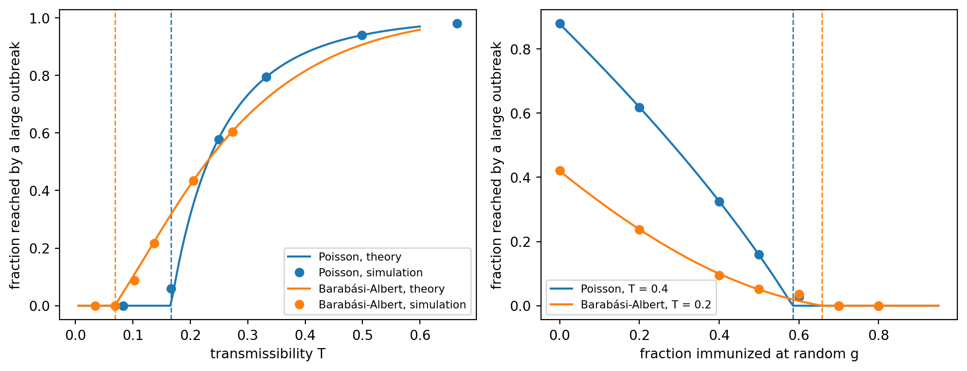
We generate configuration-model graphs with $N = 4000$ nodes from two degree sequences: Poisson with mean 6, and the degree sequence of a Barabási-Albert graph with $m = 3$. For each transmissibility, we run the Reed-Frost model from one random node and record the fraction ever infected. A run is a large outbreak if it infects more than 2% of the nodes; we average the size over large outbreaks, which is what @eq-S-percolation predicts. The theory is evaluated with the empirical degree distribution of each graph, so there is no free parameter.
```{python}
#| label: fig-sir-percolation
#| fig-cap: "Final size of SIR outbreaks on configuration-model graphs with N = 4000 and a Poisson degree sequence (ER-like) or a Barabási-Albert degree sequence (m = 3). Left: fraction of nodes reached by a large outbreak against the transmissibility T. Lines: theory of the generating-function equation; dots: Reed-Frost simulation (mean over large outbreaks, 100 runs per point). Vertical dashed lines: T_c = 1/(kappa - 1). Right: the same with a fraction g of the nodes immunized at random, at fixed T; vertical dashed lines: g_c = 1 - 1/R_0 with R_0 = T(kappa - 1)."
def percolation_S(deg, T, phi=1.0):
    """Fraction of all nodes in the giant cluster for bond occupation T and site occupation phi."""
    p = np.bincount(deg) / len(deg)
    ks = np.arange(len(p))
    mean = (ks * p).sum()
    G0 = lambda x: (p * x**ks).sum()
    G1 = lambda x: (ks[1:] * p[1:] * x ** (ks[1:] - 1)).sum() / mean
    u = 0.5
    for _ in range(20_000):
        u_new = 1 - phi * T + phi * T * G1(u)
        if abs(u_new - u) < 1e-13:
            break
        u = u_new
    return phi * (1 - G0(u))


def simple_configuration_graph(deg, seed):
    G = nx.Graph(nx.configuration_model(list(deg), seed=seed))
    G.remove_edges_from(nx.selfloop_edges(G))
    return G


N = 4000
rng = np.random.default_rng(1)
deg_poisson = rng.poisson(6, N)
deg_poisson[0] += deg_poisson.sum() % 2
deg_ba = np.array([d for _, d in nx.barabasi_albert_graph(N, 3, seed=1).degree()])
nets = {"Poisson": (deg_poisson, "C0"), "Barabási-Albert": (deg_ba, "C1")}

rng = np.random.default_rng(SEED)
n_runs, big = 100, 0.02
fig, axes = plt.subplots(1, 2, figsize=(10, 3.9))
for name, (deg, colour) in nets.items():
    G = simple_configuration_graph(deg, 1)
    k = deg.astype(float)
    kappa = (k**2).mean() / k.mean()
    Tc = 1 / (kappa - 1)
    # left panel: S against T
    T_fine = np.linspace(0.005, 0.6, 120)
    axes[0].plot(T_fine, [percolation_S(deg, T) for T in T_fine], color=colour, label=f"{name}, theory")
    axes[0].axvline(Tc, color=colour, ls="--", lw=1)
    T_sim = np.array([0.5, 1.0, 1.5, 2.0, 3.0, 4.0]) * Tc
    means = []
    for T in T_sim:
        s = np.array([run_sir_fast(G, T, 1.0, initial_infected=1, rng=rng) for _ in range(n_runs)])
        means.append(s[s > big].mean() if (s > big).any() else 0.0)
    axes[0].plot(T_sim, means, "o", color=colour, label=f"{name}, simulation")
    # right panel: random immunization at fixed T
    T = 0.4 if name == "Poisson" else 0.2
    R0 = T * (kappa - 1)
    gc = 1 - 1 / R0
    g_fine = np.linspace(0, 0.95, 100)
    axes[1].plot(g_fine, [percolation_S(deg, T, 1 - g) for g in g_fine], color=colour, label=f"{name}, T = {T}")
    axes[1].axvline(gc, color=colour, ls="--", lw=1)
    g_sim = np.array([0, 0.2, 0.4, 0.5, 0.6, 0.7, 0.8])
    means = []
    for g in g_sim:
        s = np.array([run_sir_fast(G, T, 1.0, initial_infected=1, immune=random_immunization(G, g, rng), rng=rng)
                      for _ in range(n_runs)])
        means.append(s[s > big].mean() if (s > big).any() else 0.0)
    axes[1].plot(g_sim, means, "o", color=colour)
    g_th = next(g for g in np.linspace(0, 0.99, 991) if percolation_S(deg, T, 1 - g) < 1e-3)
    print(f"{name}: kappa = {kappa:.2f}, T_c = {Tc:.3f};  T = {T}: R0 = {R0:.2f}, g_c = 1 - 1/R0 = {gc:.3f}, "
          f"theory curve falls below 0.001 at g = {g_th:.3f}")
axes[0].set_xlabel("transmissibility T")
axes[0].set_ylabel("fraction reached by a large outbreak")
axes[0].legend(fontsize=8)
axes[1].set_xlabel("fraction immunized at random g")
axes[1].set_ylabel("fraction reached by a large outbreak")
axes[1].legend(fontsize=8)
plt.tight_layout()
plt.show()
```
The simulation follows the theory without adjustment, over the whole range of $T$ and for both degree distributions: the transition is at $T_c = 1/(\kappa - 1)$, and the Barabási-Albert sequence, with a larger $\kappa$, has a transition at a transmissibility 2.4 times smaller than the Poisson one ($0.068$ against $0.166$). The finite size smooths the transition, so the points just above $T_c$ are slightly different from the curve.
## Random immunization and the herd immunity threshold
Immunizing a fraction $g$ of the nodes at random removes each node with probability $g$. On a configuration-model network this scales the mean number of onward transmissions by $1 - g$, so an outbreak is possible if
$$
(1-g)\,T\,(\kappa - 1) > 1 \quad \Longleftrightarrow \quad g < g_c = 1 - \frac{1}{R_0}, \qquad R_0 = T(\kappa - 1).
$$ {#eq-gc-network}
Here $R_0 = T(\kappa-1)$ is the mean number of secondary infections caused by a node reached along an edge in the early stage: each of its $\kappa - 1$ other edges transmits with probability $T$. This is the formula $v_c = 1 - 1/R_0$ of [SIR Extensions](../low-dimensional-dynamics/sir-extensions.qmd) for a well-mixed population, with one difference that matters: **the reproduction number now depends on the degree distribution through $\kappa$**. For a Poisson graph $\kappa - 1 = \langle k \rangle$ and $R_0 = T\langle k \rangle$, as in the homogeneous model. For a broad distribution $\kappa - 1$ is large and so is $g_c$. The right panel of @fig-sir-percolation shows the vanishing of the outbreak at the predicted $g_c$ for both networks; the output above shows that the theory curve falls to zero at the value given by @eq-gc-network.
This is the quantitative content of the first strategy of [Vaccination Strategies](vaccination-strategies.qmd), random immunization. It also explains why that page finds random vaccination so costly on the Barabási-Albert graph, while targeted vaccination of the hubs, which lowers $\kappa$, is effective [@pastor2002immunization].
::: {.callout-note}
## Exercise 1: SIR against SIS
For the continuous-time SIR model with exponential recovery, $\langle T \rangle = \lambda/(1+\lambda)$. Use @eq-Tc to show that the SIR threshold in terms of $\lambda$ is $\lambda_c^{\text{SIR}} = 1/(\kappa - 2) = \langle k \rangle/(\langle k^2 \rangle - 2\langle k \rangle)$. Evaluate it for a Poisson graph with $\langle k \rangle = 6$ and compare it with the SIS heterogeneous mean-field threshold $\lambda_c^{\text{SIS}} = \langle k \rangle/\langle k^2 \rangle$ of [Epidemic Threshold](epidemic-threshold.qmd).
:::
::: {.callout-tip collapse="true"}
## Solution
$T_c = \lambda_c/(1+\lambda_c) = 1/(\kappa-1)$ gives $\lambda_c = T_c/(1-T_c) = 1/(\kappa - 2)$, and $\kappa - 2 = (\langle k^2 \rangle - 2\langle k \rangle)/\langle k \rangle$. For the Poisson distribution $\langle k^2 \rangle = \langle k \rangle^2 + \langle k \rangle$, so $\kappa = \langle k \rangle + 1 = 7$ and $\lambda_c^{\text{SIR}} = 1/5 = 0.2$. The SIS mean-field threshold is $1/(\langle k \rangle + 1) = 1/7 \approx 0.14$. The SIR threshold is larger: in SIR the infected nodes become immune, so the infection cannot return to a node that has already had it, and a larger spreading rate is needed. The expression for SIR diverges at $\kappa = 2$, the Molloy-Reed point, below which the network has no giant component at all.
:::
::: {.callout-note}
## Exercise 2: random vaccination in a large scale-free network
A Barabási-Albert graph with $m = 3$ and $N = 10^5$ nodes has $\kappa \approx 22.2$ (compute it with `nx.barabasi_albert_graph(100_000, 3, seed=1)`). Take $T = 0.3$. Find $T_c$ and the fraction $g_c$ that must be immunized at random, and compare with a Poisson graph of mean degree 6 at the same $T$.
:::
::: {.callout-tip collapse="true"}
## Solution
$T_c = 1/(\kappa - 1) \approx 0.047$, so $T = 0.3$ is more than six times the threshold: $R_0 = T(\kappa - 1) \approx 6.4$ and $g_c = 1 - 1/R_0 \approx 0.84$. For the Poisson graph, $R_0 = 0.3 \times 6 = 1.8$ and $g_c = 1 - 1/1.8 \approx 0.44$. The same transmissibility needs almost twice the coverage on the scale-free network if the vaccinated individuals are chosen at random. The formula is for the configuration model with $N \to \infty$; the value of $g_c$ for a finite graph is lower than the one for the infinite network of the same type, but it remains large.
:::
::: {.callout-note}
## Exercise 3: random recovery times
Repeat the test for the discrete-time SIR model with $\mu = 0.2$ in place of the Reed-Frost chain. Choose $\beta$ from @eq-T-discrete so that $T = 1/3$ on the Poisson graph, run 150 simulations, and compare the mean size and the fraction of large outbreaks with the theory.
:::
::: {.callout-tip collapse="true"}
## Solution
Invert @eq-T-discrete: $\beta = T\mu/\big(1 - T(1-\mu)\big) \approx 0.0908$ for $T = 1/3$ and $\mu = 0.2$.
```python
T, mu = 1 / 3, 0.2
b = T * mu / (1 - T * (1 - mu))
G = simple_configuration_graph(deg_poisson, 1)
s = np.array([run_sir_fast(G, b, mu, initial_infected=1, rng=rng) for _ in range(150)])
print(round(b, 4), (s > 0.02).mean(), s[s > 0.02].mean(), percolation_S(deg_poisson, T))
```
The mean size of large outbreaks is 0.80 against a theoretical 0.796, so the final size agrees. The fraction of runs that become large outbreaks is lower: in 600 runs it was 0.66 for the geometric recovery times, against 0.78 for the Reed-Frost chain with the same $T$ (the percolation formula gives 0.80 for the latter). With random recovery times the probability of a large outbreak is not given by the same percolation formula, as the discussion above states. With only 150 runs this fraction fluctuates by several percentage points, so use more runs to see the difference.
:::
## What's Next?
The next page returns to Module 1 with a different extension of the SIR model: [Metapopulation Epidemics](metapopulation-epidemics.qmd), where the network connects whole populations and not individuals.