The Diffusion Equation
Module 3: Modelling with Randomness
A single walker is unpredictable. The density of many walkers obeys a deterministic partial differential equation. This page derives it from the lattice walk, following the idea of (berg1993random?).
From the walk to a PDE
Let \(P(x, t)\) be the probability that a walker is at site \(x\) at time \(t\). An unbiased walker at \(x\) at time \(t + \tau\) came from \(x - \delta\) or from \(x + \delta\), each with probability \(1/2\):
\[ P(x, t + \tau) = \tfrac{1}{2} P(x - \delta, t) + \tfrac{1}{2} P(x + \delta, t). \]
Expand the left side to first order in \(\tau\) and the right side to second order in \(\delta\):
\[ \tau \frac{\partial P}{\partial t} = \frac{\delta^2}{2} \frac{\partial^2 P}{\partial x^2} + O(\delta^4) + O(\tau^2). \]
Now let \(\delta \to 0\) and \(\tau \to 0\) while the ratio \(D = \delta^2 / (2\tau)\) stays fixed. The result is the diffusion equation
\[ \frac{\partial P}{\partial t} = D \frac{\partial^2 P}{\partial x^2} . \tag{1}\]
The limit only makes sense with \(\delta^2 \propto \tau\). If you scale \(\delta \propto \tau\) instead, the right side vanishes and nothing spreads. This is the continuum version of the \(\sqrt{t}\) law from Mean Squared Displacement. The same equation, written for a concentration, is Fick’s second law (berg1993random?).
The heat kernel
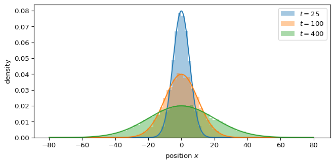
For walkers that all start at \(x = 0\), \(P(x, 0) = \delta_{\text{Dirac}}(x)\), the solution on the whole line is
\[ P(x, t) = \frac{1}{\sqrt{4\pi D t}} \exp\left(-\frac{x^2}{4Dt}\right), \tag{2}\]
a Gaussian with mean zero and variance \(2Dt\) (berg1993random?, Eq. 1.22). Its variance reproduces \(\langle x^2 \rangle = 2Dt\). The same Gaussian also follows from the binomial distribution of the walk when the number of steps is large, which is a special case of the central limit theorem.
Assumptions to remember
Equation 1 needs independent steps with finite variance and no bias. A bias adds a drift term, which gives diffusion with drift (berg1993random?). If the step variance is infinite, the limit is not a Gaussian at all; see Stable Distributions. In Module 4 the same Laplacian term appears in reaction-diffusion models.
Exercise
Check numerically that Equation 2 solves Equation 1. Evaluate heat_kernel on a grid at \(t = 10\) with \(D = 0.5\), approximate \(\partial_t P\) with a centred difference in time and \(\partial_{xx} P\) with the three-point stencil, and report the largest difference between the two sides.
Solution
from amlab.random_walks import heat_kernel

D, t, h, dt = 0.5, 10.0, 0.01, 1e-4
xg = np.arange(-10, 10, h)
dPdt = (heat_kernel(xg, t + dt, D) - heat_kernel(xg, t - dt, D)) / (2 * dt)
P = heat_kernel(xg, t, D)
d2Pdx2 = (P[2:] - 2 * P[1:-1] + P[:-2]) / h**2
print(f"max |dP/dt - D d2P/dx2| = {np.max(np.abs(dPdt[1:-1] - D * d2Pdx2)):.2e}")
print(f"max |dP/dt| = {np.max(np.abs(dPdt)):.2e}")
max |dP/dt - D d2P/dx2| = 1.58e-08
max |dP/dt| = 6.31e-03The residual is several orders of magnitude smaller than the terms themselves, as expected from discretization error alone.