Returns and Efficient Markets
Module 3: Modelling with Randomness
Reading
- Compulsory: (mantegna2000introduction?), Chapters 1 to 3.
- Recommended: (mandelbrot1963variation?); (mantegna1995scaling?).
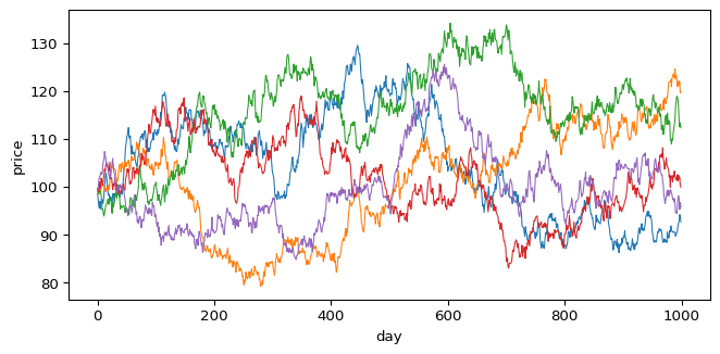
The first random walk model of prices is older than Einstein’s theory of Brownian motion. Bachelier modelled price changes on the Paris exchange as independent Gaussian increments in his 1900 thesis (bachelier1900theorie?). This session asks how well that model describes real markets.
Prices and returns
Let \(P_t\) be the closing price on day \(t\). The simple return and the log return are
\[ R_t = \frac{P_t - P_{t-1}}{P_{t-1}}, \qquad r_t = \ln \frac{P_t}{P_{t-1}} = \ln(1 + R_t). \tag{1}\]
For daily data \(|R_t|\) is usually small and \(r_t \approx R_t\). Log returns have one property that makes them the natural variable for modelling: they add over time. The log return over \(\Delta t\) days is
\[ r_t(\Delta t) = \ln \frac{P_t}{P_{t - \Delta t}} = \sum_{i=0}^{\Delta t - 1} r_{t-i} . \tag{2}\]
So \(\ln P_t\) is a random walk whose steps are the daily log returns, and everything from The Random Walk and Stable Distributions applies to it.
The random walk hypothesis
The simplest model assumes that daily log returns are independent and identically distributed, often Gaussian with mean \(\mu\) and variance \(\sigma^2\):
\[ \ln P_t = \ln P_0 + \sum_{i=1}^{t} r_i, \qquad r_i \overset{\text{iid}}{\sim} \mathcal{N}(\mu, \sigma^2). \tag{3}\]
Then \(\operatorname{Var}[r_t(\Delta t)] = \sigma^2 \Delta t\), the financial version of \(\mathrm{MSD} = 2Dt\). Bachelier’s original model used price changes instead of log returns (bachelier1900theorie?).
Efficient markets
(fama1970efficient?) calls a market efficient when prices “fully reflect” the available information. He distinguishes three forms by the information set: past prices (weak form), all public information (semi-strong form), and all information, including private information (strong form). Fama also notes that the independence assumed in Equation 3 is stronger than what efficiency requires. In a “fair game” model the deviations of returns from their expected values cannot be predicted from the information set, but they need not be independent or identically distributed (fama1970efficient?).
The practical consequence you test in the lab: under weak-form efficiency, past returns should carry no linear information about future returns.
Exercise
A price goes from 100 to 150 and then back to 100. Compute the two simple returns and the two log returns. Which of them sum to the total return over the two days?
Solution
p = np.array([100.0, 150.0, 100.0])
R = np.diff(p) / p[:-1]
r = np.diff(np.log(p))
print("simple returns:", R, "sum", R.sum())
print("log returns:   ", r.round(4), "sum", r.sum().round(12))
simple returns: [ 0.5 -0.33333333] sum 0.16666666666666669
log returns: [ 0.4055 -0.4055] sum 0.0The simple returns are \(+50\%\) and \(-33.3\%\); their sum, \(+16.7\%\), is not the true total return of \(0\). The log returns are \(\pm 0.405\) and sum to exactly \(0\).