The Order Parameter
Module 2: Synchronization and Collective Behaviour
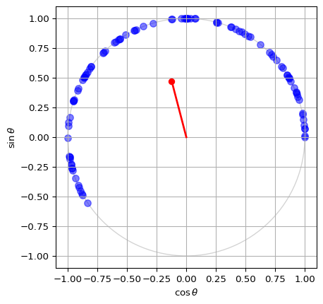
To visualize the Kuramoto model, picture each phase \(\theta_j\) as a point \(e^{i\theta_j}\) running around the unit circle in the complex plane (Strogatz 2000).
Definition
The complex order parameter is the centroid of these points:
\[ r e^{i\psi} = \frac{1}{N} \sum_{j=1}^N e^{i\theta_j}. \tag{1}\]
- \(r \in [0, 1]\) is the coherence. \(r = 1\) when all phases coincide. \(r \approx 0\) when the phases are spread around the circle.
- \(\psi\) is the mean phase, the phase of the collective rhythm.
In Figure 1 the initial phases cover only part of the circle, so the red vector has a clear length and direction. To see the vector move as the phases evolve, run the script amlab/odes_coupled/kuramoto.py. You build the same animation yourself in Animation.
Mean-field form
Multiply Equation 1 by \(e^{-i\theta_i}\) and take the imaginary part:
\[ r\sin(\psi - \theta_i) = \frac{1}{N}\sum_{j=1}^N \sin(\theta_j - \theta_i). \]
The Kuramoto model therefore becomes
\[ \dot\theta_i = \omega_i + K r \sin(\psi - \theta_i),\quad i = 1, \dots, N. \tag{2}\]
This rewriting is exact for every \(N\) (Strogatz 2000). Each oscillator no longer sees the others one by one. It sees only the mean field: it is pulled toward the mean phase \(\psi\) with effective strength \(Kr\). Computing \(r\) and \(\psi\) costs \(O(N)\) operations per step, while the double sum in the pairwise form costs \(O(N^2)\).
Feedback between coherence and coupling
Equation 2 shows why synchronization can appear spontaneously (Strogatz 2000):
- Oscillators are pulled toward \(\psi\) with strength \(Kr\).
- If more of them cluster, \(r\) grows.
- A larger \(r\) increases the pull \(Kr\), which recruits more oscillators.
The loop is opposed by the spread of natural frequencies. Oscillators whose \(|\omega_i|\) exceeds \(Kr\) cannot follow the mean field and keep drifting. The balance sets a threshold coupling \(K_c\), derived in Critical Coupling.
Exercise
Suppose the \(N\) phases are independent and uniform on \([0, 2\pi)\). Show that \(\mathbb{E}[r^2] = 1/N\). What does this imply for the value of \(r\) you measure in an incoherent simulation?
Solution
\[ r^2 = \left|\frac{1}{N}\sum_j e^{i\theta_j}\right|^2 = \frac{1}{N^2}\sum_{j,k} e^{i(\theta_j - \theta_k)}. \]
The \(N\) terms with \(j = k\) equal \(1\). For \(j \ne k\) the phases are independent, so \(\mathbb{E}[e^{i(\theta_j-\theta_k)}] = \mathbb{E}[e^{i\theta_j}]\,\mathbb{E}[e^{-i\theta_k}] = 0\). Hence \(\mathbb{E}[r^2] = N/N^2 = 1/N\). An incoherent population with \(N = 100\) shows \(r\) of order \(0.1\), not \(0\). You will see this floor in Finite-Size Effects.
Exercise
Compute \(r\) for three oscillators at phases \(0\), \(2\pi/3\) and \(4\pi/3\), and for three oscillators at \(0\), \(0\) and \(\pi\).
Solution
The first three points are the cube roots of unity, which sum to zero, so \(r = 0\). For the second set, \(e^{0} + e^{0} + e^{i\pi} = 1\), so \(r = 1/3\) and \(\psi = 0\).
References
Strogatz, Steven H. 2000. “From Kuramoto to Crawford: Exploring the Onset of Synchronization in Populations of Coupled Oscillators.” Physica D: Nonlinear Phenomena 143: 1–20.