Real networks have short paths, high clustering and, often, hubs (newman2003structure?). This session builds three models that reproduce some of these features. The first one is the simplest random graph: it serves as the null model against which you compare the others.
The model
In the Gilbert model \(G(N, p)\) every pair of nodes is joined independently with probability \(p\)(Gilbert 1959). The closely related Erdős-Rényi model \(G(N, E)\) picks a graph uniformly among all graphs with exactly \(E\) edges (Erdos and Renyi 1959). For large \(N\) the two behave the same, and both go by the name “random graph”.
Let \(c = (N-1)p\) be the mean degree. Key properties, for large \(N\) with \(c\) fixed (newman2003structure?; Newman 2018):
The degree distribution is binomial and tends to a Poisson distribution, \(p_k = e^{-c} c^k / k!\). So \(\langle k^2 \rangle = c^2 + c\).
The clustering coefficient is \(C = p = c/(N-1)\), which tends to zero as \(N\) grows.
A giant component exists if and only if \(c > 1\). This agrees with the Molloy-Reed criterion of Robustness and Percolation: \(\kappa = \langle k^2 \rangle / \langle k \rangle = c + 1 > 2\).
The fraction \(S\) of nodes in the giant component solves \(S = 1 - e^{-cS}\).
The typical distance grows like \(\ell \approx \ln N / \ln c\).
Implementation
NetworkX provides nx.erdos_renyi_graph(n, p) for \(G(N,p)\) and nx.gnm_random_graph(n, m) for \(G(N,E)\). The algorithm behind \(G(N,p)\) is short:
Select a pair of nodes \(i\) and \(j\).
Draw a random number \(r\) in \([0, 1)\). If \(r < p\), add the edge \((i, j)\).
Repeat for all pairs.
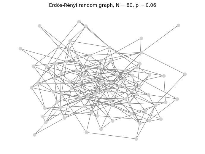
import matplotlib.pyplot as pltimport networkx as nximport numpy as npSEED =7G_random = nx.erdos_renyi_graph(n=80, p=0.06, seed=SEED)pos = nx.spring_layout(G_random, seed=SEED)nx.draw(G_random, pos=pos, node_size=60, node_color="lightgray", edge_color="gray")plt.title("Erdős-Rényi random graph, N = 80, p = 0.06")plt.show()k = np.array([d for _, d in G_random.degree()])print(f"<k> = {k.mean():.2f} (expected {(80-1) *0.06:.2f})")print(f"C = {nx.average_clustering(G_random):.3f} (expected p = 0.06)")print(f"components = {nx.number_connected_components(G_random)}")
<k> = 5.28 (expected 4.74)
C = 0.078 (expected p = 0.06)
components = 1
With \(N = 80\) a single realization fluctuates around the expected values. Increase \(N\) and watch the measured values approach the predictions.
\(G(N, p)\) vs \(G(N, E)\)
In \(G(N, E)\) you fix the number of edges instead of an edge probability. In NetworkX:
nx.gnm_random_graph(n, m) implements \(G(N, E)\) with \(E = m\);
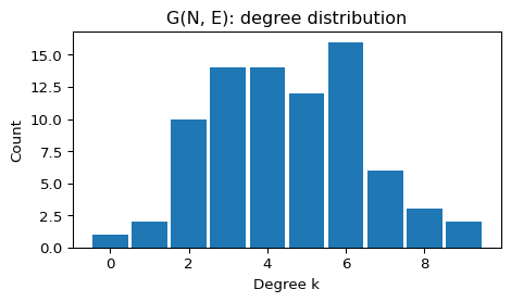
With \(N = 80\) and \(E = 180\) the mean degree is \(2E/N = 4.5\), close to the \(4.74\) of \(G(80, 0.06)\). The degree histogram has the same binomial shape.
G_gnm = nx.gnm_random_graph(n=80, m=180, seed=SEED)k_gnm = [d for _, d in G_gnm.degree()]print(f"E = {G_gnm.number_of_edges()}, <k> = {2*180/80:.2f}")plt.figure(figsize=(5, 3))plt.hist(k_gnm, bins=range(min(k_gnm), max(k_gnm) +2), align="left", rwidth=0.9)plt.xlabel("Degree k")plt.ylabel("Count")plt.title("G(N, E): degree distribution")plt.tight_layout()plt.show()
E = 180, <k> = 4.50
The giant component
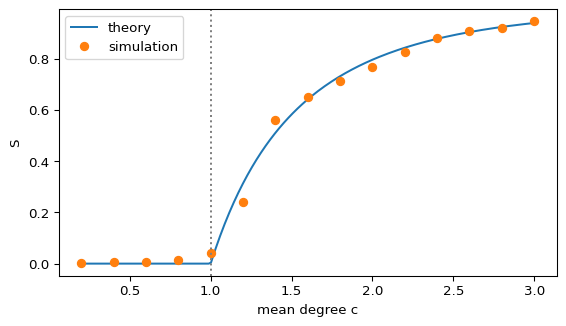
Figure 1 compares simulated graphs with the self-consistency equation \(S = 1 - e^{-cS}\).
Figure 1: Fraction of nodes in the largest component of G(N, p) with N = 2000 (dots, one graph per value) and the theoretical giant component S = 1 - exp(-cS) (line).
Near \(c = 1\) the finite graph has a largest component of size \(o(N)\) that is still visible, so the dots do not drop exactly to zero.
Exercise
Watts and Strogatz measured \(C = 0.79\) in the collaboration network of film actors, against \(C = 0.00027\) for a random graph of the same size and mean degree (Watts and Strogatz 1998, Table 1). Estimate \(C\) for a random graph with \(N = 10^6\) people and mean degree \(c = 100\). What does this say about random graphs as models of social networks?
Solution
\(C = c/(N-1) \approx 10^{-4}\). A random graph has almost no triangles, so it cannot reproduce the clustering of social networks. It does reproduce short paths: \(\ell \approx \ln 10^6 / \ln 100 = 3\). The small-world model keeps both.
Newman, Mark. 2018. Networks. 2nd ed. Oxford University Press.
Watts, Duncan J., and Steven H. Strogatz. 1998. “Collective Dynamics of ’Small-World’ Networks.”Nature 393 (6684): 440–42. https://doi.org/10.1038/30918.
Source Code
---title: "Erdős-Rényi Random Graphs"subtitle: "Module 5: Complex Networks"format: html---::: {.callout-note}## Reading- **Compulsory:** @watts1998collective; @barabasi1999emergence.- **Recommended:** @newman2018networks; @newman2003structure, Sections 4, 6 and 7.:::Real networks have short paths, high clustering and, often, hubs [@newman2003structure]. This session builds three models that reproduce some of these features. The first one is the simplest random graph: it serves as the null model against which you compare the others.## The modelIn the **Gilbert** model $G(N, p)$ every pair of nodes is joined independently with probability $p$ [@gilbert1959random]. The closely related **Erdős-Rényi** model $G(N, E)$ picks a graph uniformly among all graphs with exactly $E$ edges [@erdos1959random]. For large $N$ the two behave the same, and both go by the name "random graph".Let $c = (N-1)p$ be the mean degree. Key properties, for large $N$ with $c$ fixed [@newman2003structure, Section 4.1; @newman2018networks]:- The degree distribution is binomial and tends to a Poisson distribution, $p_k = e^{-c} c^k / k!$. So $\langle k^2 \rangle = c^2 + c$.- The clustering coefficient is $C = p = c/(N-1)$, which tends to zero as $N$ grows.- A giant component exists if and only if $c > 1$. This agrees with the Molloy-Reed criterion of [Robustness and Percolation](robustness-percolation.qmd): $\kappa = \langle k^2 \rangle / \langle k \rangle = c + 1 > 2$.- The fraction $S$ of nodes in the giant component solves $S = 1 - e^{-cS}$.- The typical distance grows like $\ell \approx \ln N / \ln c$.## ImplementationNetworkX provides `nx.erdos_renyi_graph(n, p)` for $G(N,p)$ and `nx.gnm_random_graph(n, m)` for $G(N,E)$. The algorithm behind $G(N,p)$ is short:1. Select a pair of nodes $i$ and $j$.2. Draw a random number $r$ in $[0, 1)$. If $r < p$, add the edge $(i, j)$.3. Repeat for all pairs.```{python}import matplotlib.pyplot as pltimport networkx as nximport numpy as npSEED =7G_random = nx.erdos_renyi_graph(n=80, p=0.06, seed=SEED)pos = nx.spring_layout(G_random, seed=SEED)nx.draw(G_random, pos=pos, node_size=60, node_color="lightgray", edge_color="gray")plt.title("Erdős-Rényi random graph, N = 80, p = 0.06")plt.show()k = np.array([d for _, d in G_random.degree()])print(f"<k> = {k.mean():.2f} (expected {(80-1) *0.06:.2f})")print(f"C = {nx.average_clustering(G_random):.3f} (expected p = 0.06)")print(f"components = {nx.number_connected_components(G_random)}")```With $N = 80$ a single realization fluctuates around the expected values. Increase $N$ and watch the measured values approach the predictions.::: {.callout-tip collapse="true"}## $G(N, p)$ vs $G(N, E)$In $G(N, E)$ you fix the number of edges instead of an edge probability. In NetworkX:- `nx.gnm_random_graph(n, m)` implements $G(N, E)$ with $E = m$;- `nx.erdos_renyi_graph(n, p)` (alias `nx.gnp_random_graph`) implements $G(N, p)$.:::With $N = 80$ and $E = 180$ the mean degree is $2E/N = 4.5$, close to the $4.74$ of $G(80, 0.06)$. The degree histogram has the same binomial shape.```{python}G_gnm = nx.gnm_random_graph(n=80, m=180, seed=SEED)k_gnm = [d for _, d in G_gnm.degree()]print(f"E = {G_gnm.number_of_edges()}, <k> = {2*180/80:.2f}")plt.figure(figsize=(5, 3))plt.hist(k_gnm, bins=range(min(k_gnm), max(k_gnm) +2), align="left", rwidth=0.9)plt.xlabel("Degree k")plt.ylabel("Count")plt.title("G(N, E): degree distribution")plt.tight_layout()plt.show()```## The giant component@fig-er-giant compares simulated graphs with the self-consistency equation $S = 1 - e^{-cS}$.```{python}#| label: fig-er-giant#| fig-cap: "Fraction of nodes in the largest component of G(N, p) with N = 2000 (dots, one graph per value) and the theoretical giant component S = 1 - exp(-cS) (line)."#| echo: falsefrom scipy.optimize import brentqN =2000cs = np.linspace(0.2, 3.0, 15)sim = []for i, c inenumerate(cs): G = nx.fast_gnp_random_graph(N, c / (N -1), seed=SEED + i) sim.append(len(max(nx.connected_components(G), key=len)) / N)c_fine = np.linspace(0.2, 3.0, 200)theory = [brentq(lambda s: s -1+ np.exp(-c * s), 1e-9, 1) if c >1else0for c in c_fine]fig, ax = plt.subplots(figsize=(6, 3.5))ax.plot(c_fine, theory, label="theory")ax.plot(cs, sim, "o", label="simulation")ax.axvline(1, color="grey", ls=":")ax.set_xlabel("mean degree c")ax.set_ylabel("S")ax.legend()plt.tight_layout()plt.show()```Near $c = 1$ the finite graph has a largest component of size $o(N)$ that is still visible, so the dots do not drop exactly to zero.::: {.callout-note}## ExerciseWatts and Strogatz measured $C = 0.79$ in the collaboration network of film actors, against $C = 0.00027$ for a random graph of the same size and mean degree [@watts1998collective, Table 1]. Estimate $C$ for a random graph with $N = 10^6$ people and mean degree $c = 100$. What does this say about random graphs as models of social networks?:::::: {.callout-tip collapse="true"}## Solution$C = c/(N-1) \approx 10^{-4}$. A random graph has almost no triangles, so it cannot reproduce the clustering of social networks. It does reproduce short paths: $\ell \approx \ln 10^6 / \ln 100 = 3$. The [small-world model](small-world.qmd) keeps both.:::