Van der Pol Oscillator

Module 1: Low-Dimensional Dynamics

Optional extension

This page is optional in Session 8. It applies the CDIMA pipeline to a second oscillator. Session 9 returns to it in Relaxation Oscillations.

The Van der Pol oscillator, introduced by van der Pol for electrical circuits with triodes (vanderpol1926relaxation?), is a prototypical nonlinear system that exhibits self-sustained oscillations. For a wide range of initial conditions, trajectories converge to a stable limit cycle.

In the form we will use in this course, the system is written as (Strogatz 2024, chap. 7.5):

\[\begin{aligned} \dot x &= \mu\,(y - f(x)) \\ \dot y &= -\frac{x}{\mu} \end{aligned} \tag{1}\]

where \(\mu>0\) controls the strength of the nonlinearity (and the fast-slow character for large \(\mu\)), and

\[ f(x) = \frac{x^3}{3} - x. \tag{2}\]

Nullclines and Fixed Point

The nullclines are especially simple in this model:

\[ \dot x = 0 \quad \Longrightarrow \quad y = \frac{x^3}{3} - x, \qquad \dot y = 0 \quad \Longrightarrow \quad x = 0. \]

They intersect at the origin, so \((0,0)\) is the equilibrium point. For the parameter regime used in this session, the main long-run object of interest is not the equilibrium itself, but the attracting limit cycle around it.

Figure 1: Phase plane of the Van der Pol system with mu = 3. Trajectories are shown for different initial conditions (IC as x-y, marked black). Generated with scipy.integrate.solve_ivp() and matplotlib.

Implement the Vector Field

Exercise

Complete the Van der Pol vector field Equation 1.

def van_der_pol(t, xy, mu=1.0):
    x, y = xy
    dxdt = # TODO
    dydt = # TODO
    return np.array([dxdt, dydt])

Solution

def van_der_pol(t, xy, mu=1.0):
    x, y = xy
    fx = x**3 / 3 - x
    dxdt = mu * (y - fx)
    dydt = -x / mu
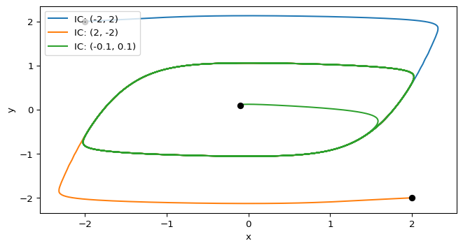
    return np.array([dxdt, dydt])

Follow the same pipeline as in CDIMA: Phase Plane: define the right-hand side, solve the initial value problem, compute nullclines, and then animate the resulting trajectory.

The Stable Limit Cycle

For every \(\mu > 0\) the Van der Pol system has a unique, stable limit cycle; this follows from Liénard’s theorem (Strogatz 2024, sec. 7.4).

Exercise

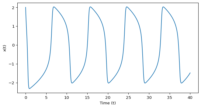
Plot this limit cycle as an \(x(t)\) against \(t\) plot for \(\mu = 3\) and the initial condition \((2, -2)\), and verify that it matches the phase plane trajectories. Figure 2 shows the expected result.

Solution

sol = solve_ivp(van_der_pol, [0, 40], (2, -2), args=(3,), t_eval=np.linspace(0, 40, 4000))
fig, ax = plt.subplots(figsize=(8, 4))
ax.plot(sol.t, sol.y[0])
ax.set_xlabel("Time (t)")
ax.set_ylabel("x(t)")
plt.show()

The maximum of \(x(t)\) is close to 2, the largest \(|x|\) on the closed orbit in Figure 1.

Figure 2: Time series of x(t) for the Van der Pol system with mu = 3 and IC: (2, -2). Generated with scipy.integrate.solve_ivp() and matplotlib.

The Role of \(\mu\)

The amplitude and period of the limit cycle depend on \(\mu\).

• For smaller \(\mu\), the oscillation looks smoother and less sharply separated into time scales.
• For larger \(\mu\), the motion develops a clear slow-fast structure.
• The trajectory spends long intervals drifting near the cubic nullcline, then jumps rapidly between branches.

This is the characteristic relaxation-oscillation picture.

What to Look For

• Different initial conditions approach the same closed orbit.
• The transient depends on the initial state, but the long-run behavior does not.
• The time trace \(x(t)\) reflects the same slow-fast pattern you see in the phase plane.

Exercise

Play with the parameter \(\mu\) (try 0.5, 1, 3 and 10) to see how it changes the shape of the limit cycle, its amplitude, its period and the transient dynamics.

Solution

The amplitude of \(x\) stays close to 2 for every \(\mu\). The period grows with \(\mu\): about 6.4 for \(\mu = 0.5\) and 19 for \(\mu = 10\). For large \(\mu\) it approaches \((3 - 2\ln 2)\mu\) (Strogatz 2024, sec. 7.5). Small \(\mu\) gives a nearly sinusoidal oscillation; large \(\mu\) gives slow drifts along the cubic nullcline and fast jumps between its branches.

for mu_test in [0.5, 1, 3, 10]:
    t_end = 40 + 30 * mu_test
    s = solve_ivp(van_der_pol, (0, t_end), [2, -2], args=(mu_test,),
                  t_eval=np.linspace(0, t_end, 200001), rtol=1e-9, atol=1e-11)
    late = s.t > t_end / 2
    x_late, t_late = s.y[0][late], s.t[late]
    up = np.where((x_late[:-1] < 0) & (x_late[1:] >= 0))[0]
    print(f"mu = {mu_test}: amplitude {x_late.max():.2f}, period {np.diff(t_late[up]).mean():.2f}, "
          f"(3 - 2 ln 2) mu = {(3 - 2 * np.log(2)) * mu_test:.2f}")

mu = 0.5: amplitude 2.00, period 6.38, (3 - 2 ln 2) mu = 0.81
mu = 1: amplitude 2.01, period 6.66, (3 - 2 ln 2) mu = 1.61
mu = 3: amplitude 2.02, period 8.86, (3 - 2 ln 2) mu = 4.84
mu = 10: amplitude 2.01, period 19.08, (3 - 2 ln 2) mu = 16.14

Next

Strogatz, Steven H. 2024. Nonlinear Dynamics and Chaos: With Applications to Physics, Biology, Chemistry, and Engineering. Chapman; Hall/CRC.