Relaxation Oscillations
Module 1: Low-Dimensional Dynamics
A relaxation oscillation alternates slow build-up with fast release. Van der Pol introduced the term for self-oscillating electrical circuits (vanderpol1926relaxation?). The standard example is his oscillator with strong nonlinearity (Strogatz 2024, sec. 7.5).
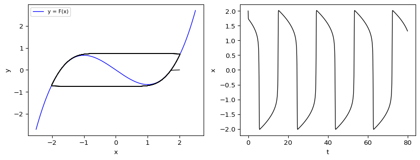
The Van der Pol oscillator for large \(\mu\)
The equation \(\ddot x + \mu(x^2 - 1)\dot x + x = 0\) has negative damping for \(|x| < 1\) and positive damping for \(|x| > 1\). With \(F(x) = x^3/3 - x\) and \(y = \dot x/\mu + F(x)\) it becomes
\[ \dot x = \mu\bigl(y - F(x)\bigr), \qquad \dot y = -\frac{x}{\mu}, \tag{1}\]
which is the form in amlab/odes_2d/van_der_pol.py (Strogatz 2024, sec. 7.5).
For \(\mu \gg 1\), \(\dot x\) is of order \(\mu\) and \(\dot y\) of order \(1/\mu\). Away from the cubic nullcline \(y = F(x)\) the trajectory jumps almost horizontally, in a time of order \(1/\mu\). On the outer branches of the cubic it creeps slowly, in a time of order \(\mu\). When it reaches a knee of the cubic (\(x = \pm 1\)) it jumps to the other branch.
The period
Strogatz computes the period from the time spent on the slow branches. On a slow branch \(y \approx F(x)\), so \(\dot y = F'(x)\dot x = (x^2 - 1)\dot x = -x/\mu\). Integrating from \(x = 2\) to \(x = 1\) and doubling for the two branches gives
\[ T \approx 2\mu \int_1^2 \frac{x^2 - 1}{x}\,dx = (3 - 2\ln 2)\,\mu \approx 1.61\,\mu, \tag{2}\]
with corrections that vanish relative to \(\mu\) as \(\mu \to \infty\) (Strogatz 2024, sec. 7.5).
Numerical check
Measure the period from upward zero crossings of \(x(t)\) and compare with Equation 2.
for mu in [5.0, 10.0, 20.0, 40.0]:
    t_end = 12 * mu
    s = solve_ivp(van_der_pol, (0, t_end), [2.0, 0.0], args=(mu,), method="LSODA",
                  t_eval=np.linspace(0, t_end, 40000), rtol=1e-8)
    x = s.y[0]
    up = s.t[1:][(x[:-1] < 0) & (x[1:] >= 0)]
    period = np.mean(np.diff(up[1:]))
    print(f"mu = {mu:4.0f}: T = {period:6.2f}, (3 - 2 ln 2) mu = {(3 - 2 * np.log(2)) * mu:6.2f}")
mu = 5: T = 11.61, (3 - 2 ln 2) mu = 8.07
mu = 10: T = 19.08, (3 - 2 ln 2) mu = 16.14
mu = 20: T = 34.68, (3 - 2 ln 2) mu = 32.27
mu = 40: T = 66.50, (3 - 2 ln 2) mu = 64.55The relative error falls as \(\mu\) grows, as expected for an asymptotic formula.
Where you meet it again
The FitzHugh-Nagumo model has the same geometry: a fast variable with a cubic nullcline and a slow recovery variable (FitzHugh-Nagumo Model). When its fixed point sits on the middle branch, the system produces relaxation oscillations; when it sits on an outer branch, the system is excitable.
Exercise
Evaluate the integral in Equation 2.
Solution
\(\int_1^2 (x - 1/x)\,dx = [x^2/2 - \ln x]_1^2 = (2 - \ln 2) - 1/2 = 3/2 - \ln 2\). Multiplying by \(2\mu\) gives \((3 - 2\ln 2)\mu\).
Next
Strogatz, Steven H. 2024. Nonlinear Dynamics and Chaos: With Applications to Physics, Biology, Chemistry, and Engineering. Chapman; Hall/CRC.