---
title: "Lévy Foraging"
subtitle: "Module 3: Modelling with Randomness"
format: html
---
::: {.callout-note}
## Reading
- **Compulsory:** @viswanathan1999optimizing, the whole letter (four pages).
- **Recommended:** @metzler2000random, for the mathematics of Lévy flights and walks.
:::
[Lévy Flights](levy-flights.qmd) showed that step lengths with density $\ell^{-\mu}$ and $1 < \mu < 3$ spread faster than Brownian motion. This page asks whether such a walk is also a *good* way to search. @viswanathan1999optimizing posed the question for a forager that looks for randomly placed targets, and the answer depends on a detail that is easy to overlook: what happens to a target after it has been found.
## What the paper does
The model is deliberately simple. Targets are placed at random with mean spacing $\lambda$, and the forager can detect a target only within a "direct vision" distance $r_v$. The forager follows two rules.
1. If a target lies within $r_v$, move straight to the nearest one.
2. Otherwise draw a direction at random and a flight length $\ell$ from $P(\ell) \propto \ell^{-\mu}$ with $1 < \mu \le 3$, and fly towards that point, stopping early if a target comes within $r_v$ on the way.
Foraging is **destructive** if a target disappears once it has been found, and **non-destructive** if it can be visited again, because it regenerates or because the forager returns to a patch. The search efficiency is the number of targets found per unit distance travelled,
$$
\eta = \frac{1}{\langle \ell \rangle\, N},
$$ {#eq-forage-eta}
where $\langle \ell \rangle$ is the mean flight length and $N$ is the mean number of flights between two successive targets [@viswanathan1999optimizing, Eq. 3]. Long flights make $\langle \ell \rangle$ large. Short flights make $N$ large, because the forager keeps searching the same neighbourhood. An optimum can only exist if these two effects balance.
The paper's mean-field argument treats all inter-target distances as equal to $\lambda$, so that a flight longer than $\lambda$ is counted as having length $\lambda$: it ends at the next target. It then uses two scaling laws for the number of flights, $N_d \sim (\lambda/r_v)^{\mu - 1}$ for destructive foraging and $N_n \sim (\lambda/r_v)^{(\mu - 1)/2}$ for non-destructive foraging. The second one is smaller because a forager can revisit the site it has just left, which is cheap for a walker that stays close to it. The paper reports three regimes.
- **Dense targets** ($\lambda \lesssim r_v$): $\langle \ell \rangle \approx \lambda$ and $N \approx 1$, so $\eta$ does not depend on $\mu$.
- **Sparse targets, destructive foraging:** $\eta$ has no maximum, and smaller $\mu$ is always better. The forager should move almost in straight lines ($\mu \to 1$).
- **Sparse targets, non-destructive foraging:** $\eta$ is maximal at $\mu_{\text{opt}} = 2 - \delta$, where the paper gives $\delta \approx 1/[\ln(\lambda/r_v)]^2$. When $\lambda/r_v$ is large but not known precisely, $\mu \approx 2$ is the robust choice.
So "the optimum is $\mu = 2$" is a statement about sparse, revisitable targets only. The paper also notes that non-destructive foraging is the more realistic case, because food often sits in patches that regenerate, and that simulations of destructive foraging on patchy and fractal target sets gave results consistent with the non-destructive case on uniformly spread targets.
## The mean-field curve
Equation (2) of the paper gives the mean flight length when flights longer than $\lambda$ are counted as $\lambda$ (I checked the closed form against numerical integration of $\ell\,\ell^{-\mu}$):
$$
\langle \ell \rangle = \frac{\mu - 1}{2 - \mu}\, r_v^{\mu - 1} \left( \lambda^{2 - \mu} - r_v^{2 - \mu} \right) + r_v^{\mu - 1} \lambda^{2 - \mu}.
$$ {#eq-forage-meanl}
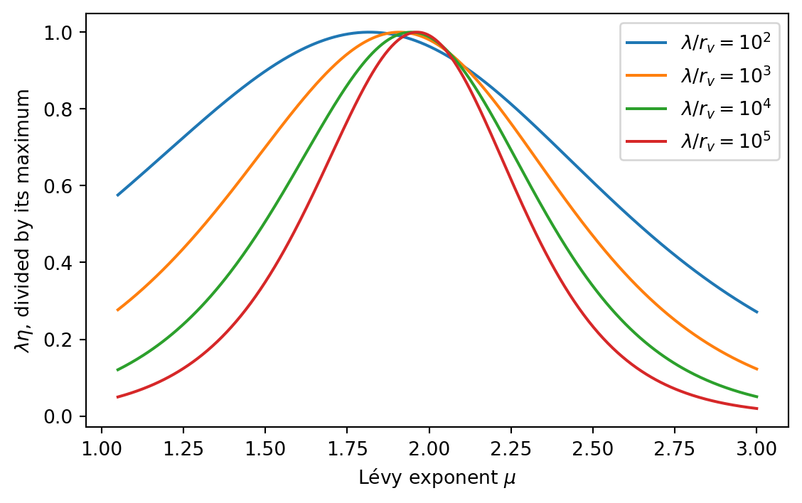
Combining it with $N_n = (\lambda / r_v)^{(\mu-1)/2}$ in @eq-forage-eta gives the efficiency curve of the figure.
```{python}
#| label: fig-forage-meanfield
#| fig-cap: "Mean-field efficiency $\\lambda\\eta$ of non-destructive foraging against the Lévy exponent $\\mu$ for four values of $\\lambda/r_v$, each curve divided by its maximum. The maximum approaches $\\mu = 2$ from below as targets become sparser."
import matplotlib.pyplot as plt
import numpy as np


def mean_flight(mu, lam, rv=1.0):
    """Mean flight length, Eq. (forage-meanl), with the cutoff at lam."""
    mu = np.asarray(mu, dtype=float)
    a = np.where(np.abs(2.0 - mu) < 1e-9, 1e-9, 2.0 - mu)  # avoids 0/0 at mu = 2
    return (mu - 1.0) * rv ** (mu - 1.0) * ((lam**a - rv**a) / a + lam**a / (mu - 1.0))


def efficiency_mean_field(mu, lam, rv=1.0):
    """eta = 1 / (N_n <l>) with N_n = (lam / rv)^((mu - 1) / 2)."""
    return 1.0 / ((lam / rv) ** ((np.asarray(mu) - 1.0) / 2.0) * mean_flight(mu, lam, rv))


mus = np.linspace(1.05, 3.0, 400)
fig, ax = plt.subplots(figsize=(6, 3.8))
for lam in [1e2, 1e3, 1e4, 1e5]:
    y = lam * efficiency_mean_field(mus, lam)
    ax.plot(mus, y / y.max(), label=rf"$\lambda/r_v = 10^{{{int(np.log10(lam))}}}$")
ax.set_xlabel(r"Lévy exponent $\mu$")
ax.set_ylabel(r"$\lambda\eta$, divided by its maximum")
ax.legend()
plt.tight_layout()
plt.show()
```
The location of the maximum approaches 2 only logarithmically in $\lambda/r_v$.
```{python}
for lam in [1e2, 1e3, 1e4, 1e6, 1e9]:
    mu_opt = mus[np.argmax(efficiency_mean_field(mus, lam))]
    delta = 2.0 - mu_opt
    print(f"lambda/r_v = {lam:7.0e}: mu_opt = {mu_opt:.3f}, "
          f"delta = {delta:.4f}, delta * ln(lambda/r_v)^2 = {delta * np.log(lam)**2:.2f}")
```
The offset $\delta$ does scale like $1/[\ln(\lambda/r_v)]^2$, as the paper states, but with a prefactor between about 4 and 5 for these formulas and not 1. The statement in the paper is an order-of-magnitude one.
## A simulation
The simulation below follows the two rules on a ring, with some choices of my own that the paper does not specify.
- Successive targets are separated by a gap drawn uniformly from $(\lambda/2, 3\lambda/2)$. Uniformly random positions would create pairs of targets closer than $r_v$, and a non-destructive forager would then bounce between them at almost no cost and inflate $\eta$.
- Flight lengths are drawn from $P(\ell) \propto \ell^{-\mu}$ with $\ell \ge r_v$ and truncated at the ring length.
- The target the forager stands on is ignored when it chooses its next move. A later return to a target counts as a new find in the non-destructive case, as in the paper's model.
```{python}
from bisect import bisect_right


def forage(mu, lam, destructive, n_found, rng, rv=1.0, n_targets=2000):
    """Targets found per unit distance for a 1D forager on a ring."""
    gaps = rng.uniform(0.5 * lam, 1.5 * lam, n_targets)
    t = np.cumsum(gaps).tolist()
    L = float(gaps.sum())
    x = rng.random() * L
    skip, found, dist = None, 0, 0.0
    while found < n_found:
        n = len(t)
        i = bisect_right(t, x)
        ahead = next(t[(i + j) % n] for j in range(3) if t[(i + j) % n] != skip)
        behind = next(t[(i - 1 - j) % n] for j in range(3) if t[(i - 1 - j) % n] != skip)
        da, db = (ahead - x) % L, (x - behind) % L
        hit = None
        if min(da, db) <= rv:  # rule 1: a target in direct vision
            hit, step = (ahead, da) if da <= db else (behind, db)
        else:  # rule 2: a new random flight
            length = min(rv * (1.0 - rng.random()) ** (-1.0 / (mu - 1.0)), L)
            if rng.random() < 0.5:
                if da - rv <= length:
                    hit, step = ahead, da
                else:
                    x, step = (x + length) % L, length
            else:
                if db - rv <= length:
                    hit, step = behind, db
                else:
                    x, step = (x - length) % L, length
        dist += step
        skip = hit
        if hit is not None:
            x = hit
            found += 1
            if destructive:
                t.remove(hit)
    return found / dist
```
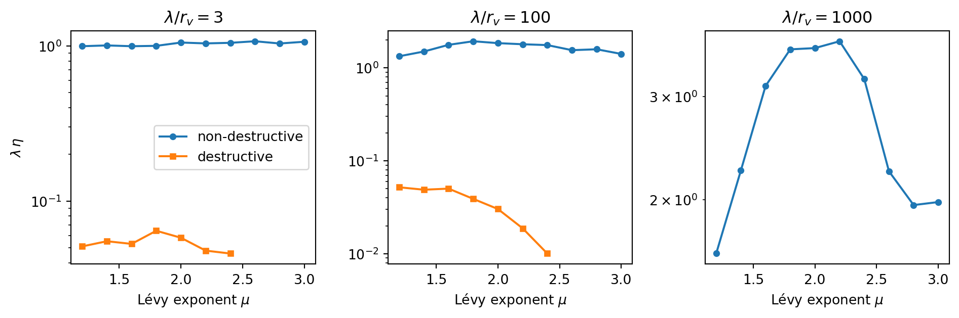
Destructive foraging with a large $\mu$ needs about $\lambda^{\mu - 1}$ flights per target, so the destructive runs use a shorter grid and fewer targets.
```{python}
#| label: fig-forage-simulation
#| fig-cap: "Simulated search efficiency $\\lambda\\eta$ of a one-dimensional forager against the Lévy exponent $\\mu$, on a logarithmic vertical axis. Left: dense targets, $\\lambda/r_v = 3$, where $\\eta$ hardly depends on $\\mu$. Centre and right: sparse targets, $\\lambda/r_v = 100$ and $1000$. For sparse targets non-destructive foraging has a maximum near $\\mu = 2$, and destructive foraging (shown for $\\mu \\le 2.4$) does not improve with $\\mu$. Each point averages independent runs."
mu_grid = np.round(np.arange(1.2, 3.01, 0.2), 1)
short_grid = mu_grid[mu_grid <= 2.4]
settings = [  # (lambda / r_v, destructive, mu values, targets per run, runs)
    (3, False, mu_grid, 300, 16), (3, True, short_grid, 100, 8),
    (100, False, mu_grid, 300, 16), (100, True, short_grid, 100, 8),
    (1000, False, mu_grid, 300, 16),
]
fig, axes = plt.subplots(1, 3, figsize=(10, 3.4))
best = {}
for lam, destructive, grid, n_found, reps in settings:
    ax = axes[[3, 100, 1000].index(lam)]
    eta = []
    for mu in grid:
        rng = np.random.default_rng(1000 * lam + int(10 * mu) + 7 * destructive)
        eta.append(lam * np.mean([forage(mu, lam, destructive, n_found, rng) for _ in range(reps)]))
    label = "destructive" if destructive else "non-destructive"
    ax.semilogy(grid, eta, "s-" if destructive else "o-", ms=4, label=label)
    ax.set_title(rf"$\lambda/r_v = {lam}$")
    ax.set_xlabel(r"Lévy exponent $\mu$")
    best[(lam, label)] = grid[int(np.argmax(eta))]
axes[0].set_ylabel(r"$\lambda\,\eta$")
axes[0].legend()
plt.tight_layout()
plt.show()

for (lam, label), mu in best.items():
    if lam >= 100:
        print(f"lambda/r_v = {lam:4d}, {label:15s}: best mu on the grid = {mu:.1f}")
```
The non-destructive curves for sparse targets are broad maxima around $\mu \approx 2$, with the peak a little below 2 for $\lambda/r_v = 100$, as the mean-field curve predicts. Destructive foraging is far less efficient at the same $\lambda$ and gets worse as $\mu$ grows, and for dense targets nothing depends on $\mu$. The qualitative picture of the paper is reproduced; the exact location of the maximum is blurred by statistical noise and by the model details listed above.
::: {.callout-note}
## Exercise
(a) Use `efficiency_mean_field` to find $\mu_{\text{opt}}$ for $\lambda/r_v = 10^2, 10^4, 10^8$ and compare with $2 - 1/[\ln(\lambda/r_v)]^2$. (b) With `forage`, estimate $\lambda\eta$ for $\lambda/r_v = 100$ at $\mu = 2$ using ring sizes of 500 and 4000 targets. Is the result sensitive to the size of the ring?
:::
::: {.callout-tip collapse="true"}
## Solution
```{python}
fine = np.linspace(1.05, 3.0, 4000)
for lam in [1e2, 1e4, 1e8]:
    mu_opt = fine[np.argmax(efficiency_mean_field(fine, lam))]
    print(f"lambda/r_v = {lam:6.0e}: mu_opt = {mu_opt:.3f}, 2 - 1/ln^2 = {2 - 1 / np.log(lam)**2:.3f}")

for n_targets in [500, 4000]:
    rng = np.random.default_rng(11)
    eta = np.mean([forage(2.0, 100, False, 300, rng, n_targets=n_targets) for _ in range(16)])
    print(f"{n_targets:5d} targets: lambda*eta = {100 * eta:.2f}")
```
The prefactor-free formula $2 - 1/\ln^2$ overshoots the mean-field optimum: the two agree only in the limit of enormous $\lambda/r_v$. The simulated efficiency agrees within about 10 % for both ring sizes, as long as the ring contains many more targets than a forager finds in one run.
:::
## What the paper does not show
- The analytical results rest on a mean-field estimate that assumes equal distances between targets. The paper also assumes a finite cutoff on the flight length, which makes the flight distribution a truncated Lévy distribution. Such a walk converges to Gaussian behaviour only after a very large number of steps, and without a cutoff the mean flight length diverges for $\mu \le 2$ [@viswanathan1999optimizing].
- The comparison with data uses published flight-length or foraging-time histograms for bumble-bees, wandering albatrosses and deer, and a published range of $2 \le \mu \le 2.5$ for amoebae. The bee data are reported with $\mu \approx 2$ at low nectar concentration and $\mu \approx 3.5$ at higher concentration, where long flights become rare and the model predicts no advantage for Lévy flights. The exponents are read from double-logarithmic plots of digitised histograms, and the letter reports neither a fitting method nor uncertainties. Given the pitfalls of that practice (see [Power Laws](power-laws.qmd) and [Fitting Power Laws Properly](power-law-fitting.qmd)), treat these exponents as consistent with $\mu \approx 2$ and not as precise estimates.
- Short-range correlations in flight directions and lengths can change the width of $P(\ell)$ but not $\mu$, according to the authors, so learning and short-term memory do not alter the long-distance result. This is an argument in the paper and is not tested here.