Lévy Flights
Module 3: Modelling with Randomness
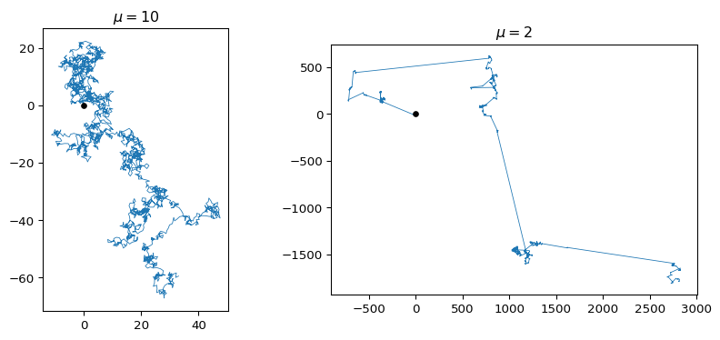
A Lévy flight is a random walk whose step lengths have a power-law distribution with infinite variance. The walk is dominated by rare long jumps, and it spreads faster than ordinary diffusion.
The model
In the plane, draw each step with a uniformly random direction and a length \(\ell\) with density
\[ p(\ell) \propto \ell^{-\mu}, \qquad \ell \ge \ell_{\min}, \]
the parametrization used by (viswanathan1999optimizing?). Three regimes follow from Power Laws and Stable Distributions:
- \(\mu \le 1\): the density cannot be normalized.
- \(1 < \mu < 3\): the step variance is infinite. The position after \(n\) steps is a sum in the domain of attraction of a stable law with index \(\alpha = \mu - 1\), so its typical size grows as \(n^{1/\alpha} = n^{1/(\mu - 1)}\). This is faster than \(n^{1/2}\).
- \(\mu > 3\): the variance is finite, the CLT applies, and you recover normal diffusion.
The mean squared displacement of a Lévy flight is infinite at every time, because a single step already has infinite variance. You measure the spreading with a quantile, such as the median distance, instead. Models that give each jump a finite speed, called Lévy walks, have a finite MSD growing as \(t^{\gamma}\) with \(\gamma > 1\) (superdiffusion) (metzler2000random?).
Trajectories
Why it matters
(viswanathan1999optimizing?) studied a searcher looking for randomly placed targets. When targets are sparse and can be revisited, the optimal choice is \(\mu \approx 2\). (metzler2000random?) review the mathematics of anomalous diffusion, including Lévy flights and walks. In finance, (mandelbrot1963variation?) proposed that price changes are stable with \(\alpha < 2\), which makes the logarithm of the price a one-dimensional Lévy flight. You test that idea in Modelling Financial Markets.
Exercise
Simulate 1000 flights of 1000 steps for \(\mu = 2.5\) and for \(\mu = 10\). Compute the median distance from the origin at each step and fit the exponent \(\nu\) in \(\text{median} \propto n^{\nu}\) over \(n \in [10, 1000]\). Compare with \(1/(\mu - 1)\) and \(1/2\).
Solution
rng = np.random.default_rng(5)
n = np.arange(10, 1001)
for mu, theory in [(2.5, 1 / 1.5), (10.0, 0.5)]:
    paths = np.array([levy_flight_2d(1000, mu=mu, rng=rng) for _ in range(1000)])
    med = np.median(np.linalg.norm(paths, axis=2), axis=0)
    nu = np.polyfit(np.log(n), np.log(med[n]), 1)[0]
    print(f"mu = {mu:4}: nu = {nu:.3f}, theory {theory:.3f}")
mu = 2.5: nu = 0.677, theory 0.667
mu = 10.0: nu = 0.501, theory 0.500The Lévy flight spreads with \(\nu \approx 2/3\), the finite-variance walk with \(\nu \approx 1/2\). Convergence to the asymptotic exponent is slow, so expect a small deviation at these sizes.