Stable Distributions
Module 3: Modelling with Randomness
The Gaussian is the limit of sums with finite variance. Sums of variables with power-law tails and infinite variance also converge, but to a different family: the Lévy stable laws (gnedenko1954limit?; mantegna2000introduction?).
Definition
A random variable \(X\) is stable if a sum of independent copies has the same shape as \(X\) itself: for every \(n\) there are constants \(a_n > 0\) and \(b_n\) with
\[ X_1 + \dots + X_n \overset{d}{=} a_n X + b_n . \]
The scale factor is always \(a_n = n^{1/\alpha}\) for some index \(0 < \alpha \le 2\) (gnedenko1954limit?). A stable law has no closed-form density in general. It is defined through its characteristic function. For the symmetric case centred at zero,
\[ \mathbb{E}\left[e^{ikX}\right] = \exp\left(-|c k|^{\alpha}\right), \tag{1}\]
with scale \(c > 0\). The general family adds a skewness parameter \(\beta \in [-1, 1]\) and a location (mantegna2000introduction?).
Key properties
- \(\alpha = 2\) gives the Gaussian with variance \(2c^2\). \(\alpha = 1\) gives the Cauchy law, with density \(c / [\pi (c^2 + x^2)]\).
- For \(\alpha < 2\) the tails are power laws, \(\Pr(|X| > x) \sim C x^{-\alpha}\) as \(x \to \infty\). The variance is infinite. For \(\alpha \le 1\) the mean does not exist either (mantegna2000introduction?).
- Generalized central limit theorem. If i.i.d. variables have tails \(\Pr(|X| > x) \sim C x^{-\alpha}\) with \(0 < \alpha < 2\), their suitably centred sums divided by \(n^{1/\alpha}\) converge to a stable law with the same \(\alpha\). If the variance is finite, the limit is Gaussian (gnedenko1954limit?).
- In the power-law notation of Power Laws, where the density decays as \(x^{-\alpha_{\text{pdf}}}\), the stable index is \(\alpha = \alpha_{\text{pdf}} - 1\). Only \(\alpha_{\text{pdf}} < 3\) leads to a non-Gaussian limit.
You can sample symmetric stable variables with the method of (chambers1976method?), implemented in amlab.random_walks.sample_symmetric_stable and in scipy.stats.levy_stable (Virtanen et al. 2020).
Cauchy against normal sample means
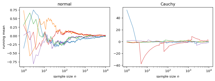
For Gaussian data the sample mean of \(n\) values has width \(\propto n^{-1/2}\). For Cauchy data, \(\alpha = 1\) and \(a_n = n\), so the sample mean \(S_n / n\) has exactly the same Cauchy law as a single observation. Averaging does not help.
Exercise
Check the scaling \(a_n = n^{1/\alpha}\) for \(\alpha = 1.5\). Draw 10000 sums of \(n\) symmetric stable variables for \(n = 1, 10, 100, 1000\), and compute the interquartile range (IQR) of each set of sums. Fit the slope of \(\log \text{IQR}\) against \(\log n\). Why do you use the IQR and not the standard deviation?
Solution
rng = np.random.default_rng(4)
ns = np.array([1, 10, 100, 1000])
iqr = []
for m in ns:
    s = sample_symmetric_stable(1.5, (10000, m), rng=rng).sum(axis=1)
    q75, q25 = np.percentile(s, [75, 25])
    iqr.append(q75 - q25)
slope = np.polyfit(np.log(ns), np.log(iqr), 1)[0]
print(f"slope {slope:.3f}, theory 1/alpha = {1 / 1.5:.3f}")
slope 0.670, theory 1/alpha = 0.667The standard deviation is infinite for \(\alpha < 2\), so its sample value is dominated by the largest draw and does not converge. Quantiles exist for every stable law.
References
Virtanen, Pauli, Ralf Gommers, Travis E. Oliphant, Matt Haberland, Tyler Reddy, David Cournapeau, Evgeni Burovski, et al. 2020. “SciPy 1.0: Fundamental Algorithms for Scientific Computing in Python.” Nature Methods 17 (3): 261–72. https://doi.org/10.1038/s41592-019-0686-2.