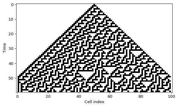
1D Cellular Automata
Module 6: Explorables and Discrete Models
Elementary cellular automata are one of the cleanest examples of emergence in a discrete system. Each cell stores a binary state, each update only depends on the three-cell neighbourhood, and repeated rule application creates nontrivial large-scale patterns (Wolfram 1983). In this lab you build the simulator yourself. The definitions are on the page Cellular Automata.
Core activity
Implement apply_rule() and simulate_ca(). On the next page you validate them on Rule 90 and reproduce the Rule 30 diagram above.
Prediction
Exercise
Rule 30 starts from a single occupied cell. Before you code, predict: how fast can the occupied region grow, in cells per step? Will the pattern stay symmetric or break symmetry quickly? Write down your answer.
Solution
The occupied region grows by at most one cell per step on each side, because each cell only sees its nearest neighbours. The figure above reaches this bound: the left and right edges move one cell per step. The pattern is not symmetric, because Rule 30 is not equal to its own reflection (the reflection is Rule 86).
What you need
numpystores the lattice, builds the rule table and updates rows.matplotlib.pyplotplots space-time diagrams and rule comparisons.matplotlib.backend_baseshandles mouse clicks in the optional interactive script on Space-Time Diagrams.
Scripts or notebooks?
Use a notebook when you want to compare several rules, inspect arrays, or save snapshots. Use a script when you want quick interaction, such as clicking on the first row and recomputing the full diagram.
Local state and neighbourhood
Let \(x_i^t \in \{0,1\}\) be the state of cell \(i\) at time \(t\). An elementary cellular automaton updates the row through a local rule
\[ x_i^{t+1} = f\big(x_{i-1}^t, x_i^t, x_{i+1}^t\big). \]
Because each neighbourhood has three binary entries, there are only \(2^3 = 8\) possible patterns. A rule is therefore an 8-entry lookup table.
Encode the rule table
By convention we order the neighbourhoods from 111 down to 000.
rule_number = 30
rule_bin = np.array([int(bit) for bit in f"{rule_number:08b}"])
For Rule 30 this produces the binary table 00011110, which tells you the output for each of the eight neighbourhoods.
Implement the local update
Exercise
Complete apply_rule(). It returns the next row, with the two edge cells kept at zero.
def apply_rule(state, rule_bin):
    new_state = np.zeros_like(state)
    for i in range(1, len(state) - 1):
        neighborhood = state[i - 1 : i + 2]
        # TODO: convert the three bits to an integer n between 0 and 7
        # TODO: look up the output (rule_bin is ordered from 111 down to 000)
        new_state[i] = # TODO
    return new_state
Hint
int("".join(neighborhood.astype(str)), 2) turns the bits [1, 1, 0] into the integer 6. Because rule_bin[0] is the output for 111 (n = 7), the output for neighbourhood n sits at index 7 - n.
Solution
def apply_rule(state, rule_bin):
    new_state = np.zeros_like(state)
    for i in range(1, len(state) - 1):
        neighborhood = state[i - 1 : i + 2]
        index = 7 - int("".join(neighborhood.astype(str)), 2)
        new_state[i] = rule_bin[index]
    return new_state
This first version keeps the boundary cells at zero because the loop only updates indices 1 through len(state) - 2. The page Boundary Conditions treats the edges properly.
Simulate many time steps
Exercise
Wrap the update in a reusable simulator that stores every row in a 2D array.
def simulate_ca(initial_state, rule_number, steps):
    rule_bin = np.array([int(bit) for bit in f"{rule_number:08b}"])
    grid = np.zeros((steps, len(initial_state)), dtype=int)
    grid[0] = initial_state

    for t in range(1, steps):
        grid[t] = # TODO: apply the rule to the previous row

    return grid
Solution
def simulate_ca(initial_state, rule_number, steps):
    rule_bin = np.array([int(bit) for bit in f"{rule_number:08b}"])
    grid = np.zeros((steps, len(initial_state)), dtype=int)
    grid[0] = initial_state
    for t in range(1, steps):
        grid[t] = apply_rule(grid[t - 1], rule_bin)
    return grid
Next
Wolfram, Stephen. 1983. “Statistical Mechanics of Cellular Automata.” Reviews of Modern Physics 55 (3): 601–44. https://doi.org/10.1103/RevModPhys.55.601.