Every simulation runs on a finite lattice, so you must decide what the edge cells see. This page compares periodic and fixed boundaries and shows how the finite size shapes the long-run behaviour. The reference code is amlab/cellular_automata/elementary.py.
Core activity
Add a boundary argument to your simulator, compare periodic and fixed-zero edges for Rules 90 and 184, and measure the period of Rule 30 on small rings.
Prediction
Exercise
Before you code, answer two questions. On a ring of \(N\) cells there are \(2^N\) possible rows. What does this imply for the long-run behaviour of any rule? Which rule, 90 or 184, will be affected more by fixed-zero edges?
Solution
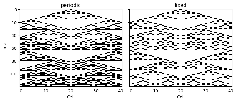
After at most \(2^N\) steps some row must repeat, and from then on the evolution cycles. So every orbit on a ring is eventually periodic, whatever the rule. Both rules change once the pattern reaches the edges, but Rule 184 changes qualitatively: it conserves the number of 1s on a ring, and fixed-zero edges let the 1s leave at the right end, so the road empties. The experiments below show both effects.
Implementation
With periodic boundaries the left neighbour of cell 0 is cell \(N-1\). np.roll gives both neighbours of every cell in one line, and the three bits give the index into the rule table.
Exercise
Complete step() so that it supports periodic and fixed-zero boundaries.
def step(state, rule, boundary="periodic"): table = np.array([(rule >> n) &1for n inrange(8)]) # entry n: output for neighbourhood nif boundary =="periodic": left, right =# TODO: use np.rollelse: padded =# TODO: add one ghost cell with value 0 at each end left, right = padded[:-2], padded[2:]return table[4* left +2* state + right]
Solution
def step(state, rule, boundary="periodic"): table = np.array([(rule >> n) &1for n inrange(8)])if boundary =="periodic": left, right = np.roll(state, 1), np.roll(state, -1)else: padded = np.concatenate(([0], state, [0])) left, right = padded[:-2], padded[2:]return table[4* left +2* state + right]
This is step_eca() in the reference module.
Validation
Far from the edges, the two boundary choices must give the same rows. Check it on a wide lattice where the pattern never reaches the edges:
import numpy as npimport matplotlib.pyplot as pltfrom amlab.cellular_automata.elementary import simulate_eca, single_seed, random_row, transient_and_perioda = simulate_eca(single_seed(201), 30, 80, boundary="periodic")b = simulate_eca(single_seed(201), 30, 80, boundary="fixed")print("Identical while the pattern is far from the edges:", np.array_equal(a, b))
Identical while the pattern is far from the edges: True
Experiment: patterns that reach the edge
Figure 1: Rule 90 from a single seed on 41 cells for 120 steps. Left: periodic, the two fronts meet on the other side of the ring. Right: fixed zero edges.
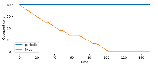
Figure 2: Number of occupied cells under Rule 184, from the same random row of 100 cells with density 0.4.
With fixed-zero edges, Rule 184 moves particles out through the right edge and brings in nothing at the left, so the road empties. With periodic edges the count is conserved. For a traffic model the boundary decides whether you model a closed ring road or an open road segment.
Experiment: every orbit on a ring is periodic
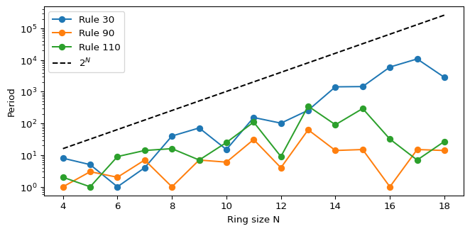
A ring of \(N\) cells has \(2^N\) configurations. After at most \(2^N\) steps some row must repeat, and from then on the evolution cycles. transient_and_period() records every row until the first repeat.
Figure 3: Period of the orbit that starts from a single seed on a ring of N cells. Logarithmic vertical axis. The dashed line is the bound 2^N.
Interpretation
Any finite simulation is eventually periodic. For Rule 30 the period grows quickly with \(N\), so on a lattice of a few hundred cells you never see the repeat. The class 3 behaviour you observe is a transient of a finite system.
Rule 90 has short periods, and for some sizes the seed dies out completely. Find the sizes where the period is 1 in the output of transient_and_period().
A boundary is part of the model. Report it together with the rule and the lattice size.
Limitations
The period depends on the initial row, not only on the rule and \(N\). The figure uses a single seed.
Storing every row limits transient_and_period() to rings of about 20 cells.
Optional extension
Exercise
Optional. Replace the ghost value 0 by 1, or use reflecting edges (the ghost copies the edge cell). Track the number of occupied cells for Rules 184, 90 and 30. Which rules change their long-run behaviour?
Solution
Rule 184 is the rule that changes most. With ghost value 1 the left ghost feeds new 1s into the lattice, the right ghost blocks the exit, and the row fills up completely. With reflecting edges no 1 can leave or enter, so the count is conserved and all 1s pile up at the right end as one jam. Rules 90 and 30 keep an irregular pattern whose number of occupied cells fluctuates from step to step, for every boundary choice. The single values printed below are snapshots of these fluctuations, not steady states.
from amlab.cellular_automata.elementary import rule_table, step_ecadef step_reflect(state, rule): table = rule_table(rule) padded = np.concatenate((state[:1], state, state[-1:]))return table[4* padded[:-2] +2* state + padded[2:]]updates = {"ghost 0": lambda s, r: step_eca(s, r, boundary="fixed", fixed_value=0),"ghost 1": lambda s, r: step_eca(s, r, boundary="fixed", fixed_value=1),"reflecting": step_reflect,}row = random_row(100, 0.4, seed=2)for rule in (184, 90, 30):for name, update in updates.items(): state = row.copy()for t inrange(300): state = update(state, rule)print(f"Rule {rule:3d}, {name:10s}: {int(state.sum()):3d} occupied cells after 300 steps")
---title: "Boundary Conditions"subtitle: "Module 6: Explorables and Discrete Models"format: html---Every simulation runs on a finite lattice, so you must decide what the edge cells see. This page compares periodic and fixed boundaries and shows how the finite size shapes the long-run behaviour. The reference code is [amlab/cellular_automata/elementary.py](../../amlab/cellular_automata/elementary.py).::: {.callout-important}## Core activityAdd a `boundary` argument to your simulator, compare periodic and fixed-zero edges for Rules 90 and 184, and measure the period of Rule 30 on small rings.:::## Prediction::: {.callout-note}## ExerciseBefore you code, answer two questions. On a ring of $N$ cells there are $2^N$ possible rows. What does this imply for the long-run behaviour of *any* rule? Which rule, 90 or 184, will be affected more by fixed-zero edges?:::::: {.callout-tip collapse="true"}## SolutionAfter at most $2^N$ steps some row must repeat, and from then on the evolution cycles. So every orbit on a ring is eventually periodic, whatever the rule. Both rules change once the pattern reaches the edges, but Rule 184 changes qualitatively: it conserves the number of 1s on a ring, and fixed-zero edges let the 1s leave at the right end, so the road empties. The experiments below show both effects.:::## ImplementationWith periodic boundaries the left neighbour of cell 0 is cell $N-1$. `np.roll` gives both neighbours of every cell in one line, and the three bits give the index into the rule table.::: {.callout-note}## ExerciseComplete `step()` so that it supports periodic and fixed-zero boundaries.```pythondef step(state, rule, boundary="periodic"): table = np.array([(rule >> n) &1for n inrange(8)]) # entry n: output for neighbourhood nif boundary =="periodic": left, right =# TODO: use np.rollelse: padded =# TODO: add one ghost cell with value 0 at each end left, right = padded[:-2], padded[2:]return table[4* left +2* state + right]```:::::: {.callout-tip collapse="true"}## Solution```pythondef step(state, rule, boundary="periodic"): table = np.array([(rule >> n) &1for n inrange(8)])if boundary =="periodic": left, right = np.roll(state, 1), np.roll(state, -1)else: padded = np.concatenate(([0], state, [0])) left, right = padded[:-2], padded[2:]return table[4* left +2* state + right]```This is `step_eca()` in the reference module.:::## ValidationFar from the edges, the two boundary choices must give the same rows. Check it on a wide lattice where the pattern never reaches the edges:```{python}import numpy as npimport matplotlib.pyplot as pltfrom amlab.cellular_automata.elementary import simulate_eca, single_seed, random_row, transient_and_perioda = simulate_eca(single_seed(201), 30, 80, boundary="periodic")b = simulate_eca(single_seed(201), 30, 80, boundary="fixed")print("Identical while the pattern is far from the edges:", np.array_equal(a, b))```## Experiment: patterns that reach the edge```{python}#| echo: false#| label: fig-boundary-rule90#| fig-cap: 'Rule 90 from a single seed on 41 cells for 120 steps. Left: periodic, the two fronts meet on the other side of the ring. Right: fixed zero edges.'#| fig-width: 8#| fig-height: 3.5fig, axes = plt.subplots(1, 2, figsize=(8, 3.5), sharey=True)for ax, bc inzip(axes, ("periodic", "fixed")): ax.imshow(simulate_eca(single_seed(41), 90, 120, boundary=bc), cmap="binary", interpolation="nearest", aspect="auto") ax.set_title(bc) ax.set_xlabel("Cell")axes[0].set_ylabel("Time")plt.tight_layout()plt.show()``````{python}#| echo: false#| label: fig-boundary-rule184#| fig-cap: 'Number of occupied cells under Rule 184, from the same random row of 100 cells with density 0.4.'#| fig-width: 7#| fig-height: 3row = random_row(100, 0.4, seed=2)fig, ax = plt.subplots(figsize=(7, 3))for bc in ("periodic", "fixed"): ax.plot(simulate_eca(row, 184, 150, boundary=bc).sum(axis=1), label=bc)ax.set_xlabel("Time")ax.set_ylabel("Occupied cells")ax.legend()plt.tight_layout()plt.show()```With fixed-zero edges, Rule 184 moves particles out through the right edge and brings in nothing at the left, so the road empties. With periodic edges the count is conserved. For a traffic model the boundary decides whether you model a closed ring road or an open road segment.## Experiment: every orbit on a ring is periodicA ring of $N$ cells has $2^N$ configurations. After at most $2^N$ steps some row must repeat, and from then on the evolution cycles. `transient_and_period()` records every row until the first repeat.```{python}#| echo: false#| label: fig-ring-period#| fig-cap: 'Period of the orbit that starts from a single seed on a ring of N cells. Logarithmic vertical axis. The dashed line is the bound 2^N.'#| fig-width: 7#| fig-height: 3.5sizes = np.arange(4, 19)fig, ax = plt.subplots(figsize=(7, 3.5))for rule in (30, 90, 110): periods = [transient_and_period(single_seed(n), rule)[1] for n in sizes] ax.semilogy(sizes, periods, marker="o", label=f"Rule {rule}")ax.semilogy(sizes, 2.0** sizes, "k--", label=r"$2^N$")ax.set_xlabel("Ring size N")ax.set_ylabel("Period")ax.legend()plt.tight_layout()plt.show()```## Interpretation- Any finite simulation is eventually periodic. For Rule 30 the period grows quickly with $N$, so on a lattice of a few hundred cells you never see the repeat. The class 3 behaviour you observe is a transient of a finite system.- Rule 90 has short periods, and for some sizes the seed dies out completely. Find the sizes where the period is 1 in the output of `transient_and_period()`.- A boundary is part of the model. Report it together with the rule and the lattice size.## Limitations- The period depends on the initial row, not only on the rule and $N$. The figure uses a single seed.- Storing every row limits `transient_and_period()` to rings of about 20 cells.## Optional extension::: {.callout-note}## ExerciseOptional. Replace the ghost value 0 by 1, or use reflecting edges (the ghost copies the edge cell). Track the number of occupied cells for Rules 184, 90 and 30. Which rules change their long-run behaviour?:::::: {.callout-tip collapse="true"}## SolutionRule 184 is the rule that changes most. With ghost value 1 the left ghost feeds new 1s into the lattice, the right ghost blocks the exit, and the row fills up completely. With reflecting edges no 1 can leave or enter, so the count is conserved and all 1s pile up at the right end as one jam. Rules 90 and 30 keep an irregular pattern whose number of occupied cells fluctuates from step to step, for every boundary choice. The single values printed below are snapshots of these fluctuations, not steady states.```{python}from amlab.cellular_automata.elementary import rule_table, step_ecadef step_reflect(state, rule): table = rule_table(rule) padded = np.concatenate((state[:1], state, state[-1:]))return table[4* padded[:-2] +2* state + padded[2:]]updates = {"ghost 0": lambda s, r: step_eca(s, r, boundary="fixed", fixed_value=0),"ghost 1": lambda s, r: step_eca(s, r, boundary="fixed", fixed_value=1),"reflecting": step_reflect,}row = random_row(100, 0.4, seed=2)for rule in (184, 90, 30):for name, update in updates.items(): state = row.copy()for t inrange(300): state = update(state, rule)print(f"Rule {rule:3d}, {name:10s}: {int(state.sum()):3d} occupied cells after 300 steps")```:::## Next