Game of Life

Module 6: Explorables and Discrete Models

Conway’s Game of Life is a two-dimensional cellular automaton on a square lattice with the Moore neighbourhood of eight cells. Martin Gardner introduced it to a wide audience in 1970 (gardner1970life?). The rules are:

• Birth: a dead cell with exactly 3 live neighbours becomes alive.
• Survival: a live cell with 2 or 3 live neighbours stays alive.
• Death: every other cell is dead in the next generation.

In the notation for “life-like” rules this is B3/S23. Berlekamp, Conway and Guy outlined a proof that the Game of Life can simulate a universal computer (berlekamp1982winning?). Reference code: amlab/cellular_automata/life.py.

Core activity

Implement one generation of the Game of Life with periodic boundaries, validate it on a blinker and a glider, and classify the small patterns below as still lifes, oscillators or spaceships. The page Random Soups then follows a random initial grid.

Prediction

Exercise

Before you code, take a horizontal row of three live cells (the blinker). Apply the rules by hand for two generations. What do you get?

Solution

The two end cells have one live neighbour each, so they die. The centre cell has two and survives. The cells directly above and below the centre have three live neighbours, so they are born. After one generation you get a vertical row of three cells. The same argument turned by 90 degrees gives the horizontal row back after two generations. The blinker is an oscillator with period 2.

Implementation

Count the live neighbours of every cell by adding the eight shifted copies of the grid. Then apply birth and survival as boolean masks.

Exercise

Complete life_step() for a grid with periodic boundaries.

def life_step(grid):
    neighbours = np.zeros_like(grid)
    for dy in (-1, 0, 1):
        for dx in (-1, 0, 1):
            if dy or dx:
                neighbours += # TODO: grid shifted by (dy, dx) with np.roll, periodic
    born = # TODO: dead and exactly 3 neighbours
    survive = # TODO: alive and 2 or 3 neighbours
    return (born | survive).astype(grid.dtype)

Solution

def life_step(grid):
    neighbours = np.zeros_like(grid)
    for dy in (-1, 0, 1):
        for dx in (-1, 0, 1):
            if dy or dx:
                neighbours += np.roll(np.roll(grid, dy, axis=0), dx, axis=1)
    born = (grid == 0) & (neighbours == 3)
    survive = (grid == 1) & ((neighbours == 2) | (neighbours == 3))
    return (born | survive).astype(grid.dtype)

Validation

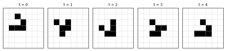
A blinker has period 2. A glider returns to its shape after 4 generations, shifted by one cell diagonally (gardner1970life?). period_and_shift() checks both.

import numpy as np
import matplotlib.pyplot as plt
from amlab.cellular_automata.life import PATTERNS, place, life_step, simulate_life, period_and_shift

for name in PATTERNS:
    period, shift = period_and_shift(place((24, 24), name, 10, 10))
    kind = "spaceship" if shift != (0, 0) else ("still life" if period == 1 else "oscillator")
    print(f"{name:8s} period {period}, shift {shift}: {kind}")

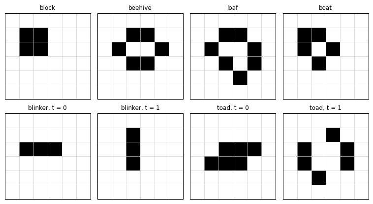
block    period 1, shift (0, 0): still life
beehive  period 1, shift (0, 0): still life
loaf     period 1, shift (0, 0): still life
boat     period 1, shift (0, 0): still life
blinker  period 2, shift (0, 0): oscillator
toad     period 2, shift (0, 0): oscillator
beacon   period 2, shift (0, 0): oscillator
glider   period 4, shift (1, 1): spaceship

Experiment: the pattern zoo

Figure 1: Top row: still lifes (block, beehive, loaf, boat). Bottom row: two generations of the period-2 oscillators blinker and toad.

Figure 2: Five generations of a glider. At t = 4 the glider has the shape of t = 0, moved one cell down and one cell right.

Interpretation

• Gliders move at one cell every four generations along a diagonal. On a periodic grid a glider can come back and collide with debris, so the final state depends on the grid size.

Exercise

Place two gliders on a \(40 \times 40\) periodic grid so that they collide. Simulate 200 generations. What remains after the collision?

Solution

glider = PATTERNS["glider"]
g = np.zeros((40, 40), dtype=np.uint8)
g[5:8, 5:8] = glider                      # moves down and right
g[5:8, 25:28] = glider[:, ::-1]           # mirrored: moves down and left
final = simulate_life(g, 200)[-1]
print("Live cells after 200 generations:", int(final.sum()))

Live cells after 200 generations: 8

The outcome depends on the relative position and phase of the gliders: they can annihilate, leave a still life or oscillators, or produce new gliders. Shift one glider by one cell and compare.

Next