import numpy as np
import matplotlib.pyplot as plt
from amlab.cellular_automata.life import life_stepRandom Soups
Module 6: Explorables and Discrete Models
A random initial grid in the Game of Life is called a soup. This page follows one soup for 300 generations and then changes the birth and survival rules. You need life_step() from the page Game of Life.
Experiment: a random soup
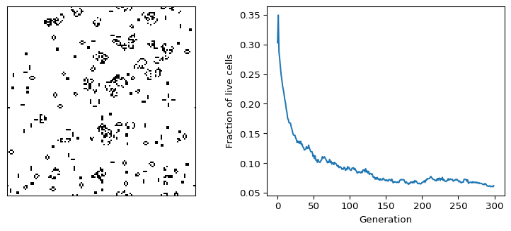
Start from a random grid and track the fraction of live cells.
Interpretation
- After a brief jump in the first generation, the density falls quickly over about 50 generations and then decays slowly. The snapshot shows mostly still lifes and blinkers, plus a few regions that are still active.
Limitations
- A finite periodic grid can only show a finite part of the Game of Life. Patterns that grow without bound need a larger or adaptive grid.
- The density curve depends on the initial fraction of live cells and on the seed. Average over several seeds before you draw conclusions.
Optional extension
Exercise
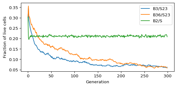
Optional. Change the rule to B36/S23 or to B2/S (birth with 2 neighbours, no survival) by editing the birth and survival masks. Repeat the random-soup experiment and compare the density curves.
Solution
B36/S23 (HighLife) adds birth with 6 neighbours. Its density curve stays above the Game of Life for the first 100 generations or so and then decays to a similar low value. B2/S (Seeds) behaves differently: every live cell dies after one generation, yet the density settles near 0.21 and the grid stays active everywhere.
from amlab.cellular_automata.life import count_neighbours


def life_like_step(grid, birth, survive):
    n = count_neighbours(grid)
    born = (grid == 0) & np.isin(n, birth)
    stay = (grid == 1) & np.isin(n, survive)
    return (born | stay).astype(grid.dtype)


fig, ax = plt.subplots(figsize=(6, 3))
for name, birth, survive in (("B3/S23", [3], [2, 3]), ("B36/S23", [3, 6], [2, 3]), ("B2/S", [2], [])):
    rng = np.random.default_rng(1)
    g = (rng.random((128, 128)) < 0.3).astype(np.uint8)
    density = []
    for t in range(300):
        density.append(g.mean())
        g = life_like_step(g, birth, survive)
    ax.plot(density, label=name)
ax.set_xlabel("Generation")
ax.set_ylabel("Fraction of live cells")
ax.legend()
plt.tight_layout()
plt.show()