amlab.finance.load_prices() reads the frozen file data/finance/prices.csv (columns date,close) when it is present in the repository. If the file is missing, it prints a warning and returns a synthetic GARCH(1,1) series with Student-t innovations and a fixed seed (bollerslev1986generalized?). The synthetic series is not market data. Check the printed message below before you interpret any number. The file format is described in data/finance/README.md.
Prediction
Exercise
Before you run any code, write down your answers:
What order of magnitude do you expect for the standard deviation of daily log returns of a stock index: 0.01 %, 1 % or 10 %?
If the market is weak-form efficient, what should the autocorrelation of \(r_t\) at lag 1 be?
Should the autocorrelation of \(|r_t|\) at lag 1 be zero too?
Solution
About 1 %. A typical stock index moves by roughly one percent on an ordinary day.
Close to zero. A clear linear correlation would let you forecast tomorrow’s return from today’s.
No. Efficiency says nothing about the size of the moves. Large moves tend to follow large moves (volatility clustering), so the autocorrelation of \(|r_t|\) is positive (cont2001empirical?). You check both answers below.
Core activity: load the data and compute log returns
import matplotlib.pyplot as pltimport numpy as npfrom amlab.finance import load_pricesdf = load_prices()print(df.head())print("source:", df.attrs["source"])
WARNING: data/finance/prices.csv not found. Using a SYNTHETIC GARCH(1,1) series with Student-t innovations (seed 2026). These are not market data. See data/finance/README.md.
        date       close
0 2006-01-02  100.000000
1 2006-01-03   99.463112
2 2006-01-04  100.264735
3 2006-01-05  100.064835
4 2006-01-06   99.944151
source: synthetic
Exercise
Write a function that returns the log returns \(r_t = \ln(P_t / P_{t-1})\) of a price array.
def log_returns(prices):"""Log returns of a 1D array of positive prices."""# TODO: take the logarithm of the prices and difference itreturn ...
Solution
def log_returns(prices):"""Log returns of a 1D array of positive prices."""return np.diff(np.log(np.asarray(prices, dtype=float)))prices = df["close"].to_numpy()dates = df["date"].to_numpy()r = log_returns(prices)print(f"{r.size} returns, mean {r.mean():.2e}, std {r.std():.4f}")
5000 returns, mean -1.09e-04, std 0.0091
The same function is available as amlab.finance.log_returns.
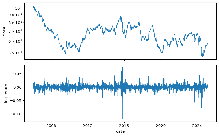
Figure 1: Closing price (log scale) and daily log returns of the lab series. Check the printed source above: if it says synthetic, these are simulated data.
Experiment: autocorrelation of returns and absolute returns
Under the null hypothesis of i.i.d. returns, sample autocorrelations are approximately normal with standard deviation \(1/\sqrt{n}\), so values outside \(\pm 2/\sqrt{n}\) are unusual.
Exercise
Complete the function below. Then compute the sample autocorrelation of \(r_t\) and of \(|r_t|\) for lags 1 to 50 and plot both with the \(\pm 2/\sqrt{n}\) band.
def autocorrelation(x, max_lag):"""Sample autocorrelation at lags 0..max_lag.""" x = x - x.mean()# TODO: for each lag k, compute sum(x[:-k] * x[k:]) / sum(x * x)return ...
Solution
Lag 0 needs care, because x[:-0] is empty. Slice with x[: x.size - k] instead.
def autocorrelation(x, max_lag):"""Sample autocorrelation at lags 0..max_lag.""" x = x - x.mean()return np.array([np.sum(x[: x.size - k] * x[k:]) / np.sum(x * x) for k inrange(max_lag +1)])
The same function is available as amlab.finance.autocorrelation, which the plot below uses.
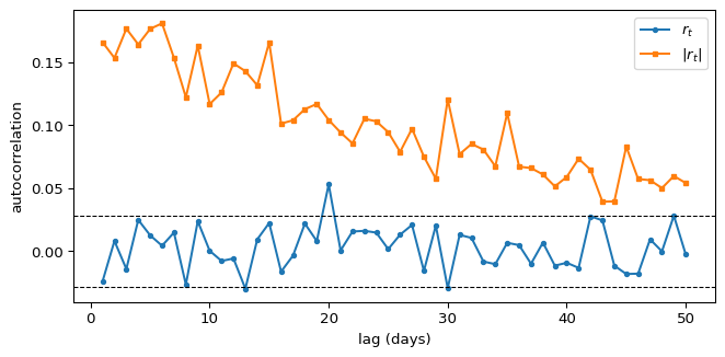
Figure 2: Sample autocorrelation of log returns and of absolute log returns. The dashed lines are \(\pm 2/\sqrt{n}\).
lag 1: r -0.024, |r| 0.166, band 0.028
Interpretation
Compare with your predictions. For market data (cont2001empirical?) reports insignificant linear autocorrelation of daily returns and a positive, slowly decaying autocorrelation of absolute returns. If your plot shows the same pattern, the returns are close to uncorrelated but they are not independent. The strong form of the random walk hypothesis, i.i.d. returns, fails.
Limitations
The \(\pm 2/\sqrt{n}\) band assumes i.i.d. data. With volatility clustering the true spread of the sample autocorrelation of \(r_t\) is wider, so a few crossings are not strong evidence (cont2001empirical?).
Closing prices that are not adjusted for dividends and splits create artificial jumps. Check the source of the frozen file.
Weekends and holidays are skipped, so a “daily” return sometimes covers three or more calendar days.
Optional extension
Exercise
Compute a 60-day rolling standard deviation of \(r_t\) with pandas.Series(r).rolling(60).std() and plot it. Mark the periods with the highest volatility. Do large returns cluster in those periods?
Solution
Shade the days where the rolling volatility is in its top 10 % and overlay the largest 1 % of absolute returns. If most of the large returns fall inside the shaded periods, they cluster.
import pandas as pdvol = pd.Series(r).rolling(60).std().to_numpy()high = vol > np.nanquantile(vol, 0.9)big = np.abs(r) > np.quantile(np.abs(r), 0.99)fig, ax = plt.subplots(figsize=(8, 3))ax.plot(dates[1:], vol, lw=0.8)ax.fill_between(dates[1:], 0, np.nanmax(vol), where=high, color="grey", alpha=0.3)ax.plot(dates[1:][big], vol[big], "r.", ms=4)ax.set_ylabel("60-day rolling std")plt.tight_layout()plt.show()print(f"share of the largest returns in high-volatility periods: {np.mean(high[big]):.2f} (about 0.10 without clustering)")
Source Code
---title: "Loading Prices and Computing Returns"subtitle: "Module 3: Modelling with Randomness"format: html---In this laboratory you test the random walk model of [Returns and Efficient Markets](efficient-markets.qmd) on a daily price series. The lab has five pages: this one (returns and autocorrelation), [Normality Tests](normality-tests.qmd), [Calibrated KS Test](ks-bootstrap.qmd), [Tail Exponent](tail-exponent.qmd) and [Scaling of Returns in Data](return-scaling-lab.qmd).::: {.callout-note}## Reading- **Recommended:** @cont2001empirical, Sections 2 and 5.:::::: {.callout-warning}## Which data you are using`amlab.finance.load_prices()` reads the frozen file `data/finance/prices.csv` (columns `date,close`) when it is present in the repository. If the file is missing, it prints a warning and returns a **synthetic** GARCH(1,1) series with Student-t innovations and a fixed seed [@bollerslev1986generalized]. The synthetic series is not market data. Check the printed message below before you interpret any number. The file format is described in `data/finance/README.md`.:::## Prediction::: {.callout-note}## ExerciseBefore you run any code, write down your answers:- What order of magnitude do you expect for the standard deviation of daily log returns of a stock index: 0.01 %, 1 % or 10 %?- If the market is weak-form efficient, what should the autocorrelation of $r_t$ at lag 1 be?- Should the autocorrelation of $|r_t|$ at lag 1 be zero too?:::::: {.callout-tip collapse="true"}## Solution- About 1 %. A typical stock index moves by roughly one percent on an ordinary day.- Close to zero. A clear linear correlation would let you forecast tomorrow's return from today's.- No. Efficiency says nothing about the size of the moves. Large moves tend to follow large moves (volatility clustering), so the autocorrelation of $|r_t|$ is positive [@cont2001empirical]. You check both answers below.:::## Core activity: load the data and compute log returns```{python}import matplotlib.pyplot as pltimport numpy as npfrom amlab.finance import load_pricesdf = load_prices()print(df.head())print("source:", df.attrs["source"])```::: {.callout-note}## ExerciseWrite a function that returns the log returns $r_t = \ln(P_t / P_{t-1})$ of a price array.```pythondef log_returns(prices):"""Log returns of a 1D array of positive prices."""# TODO: take the logarithm of the prices and difference itreturn ...```:::::: {.callout-tip collapse="true"}## Solution```{python}def log_returns(prices):"""Log returns of a 1D array of positive prices."""return np.diff(np.log(np.asarray(prices, dtype=float)))prices = df["close"].to_numpy()dates = df["date"].to_numpy()r = log_returns(prices)print(f"{r.size} returns, mean {r.mean():.2e}, std {r.std():.4f}")```The same function is available as `amlab.finance.log_returns`.:::## ValidationTwo checks catch most mistakes:- There is one return fewer than there are prices.- Log returns add up: $\sum_t r_t = \ln(P_T / P_0)$.```{python}assert r.size == prices.size -1assert np.isclose(r.sum(), np.log(prices[-1] / prices[0]))print("checks passed")```## Experiment: plot prices and returns```{python}#| label: fig-lab-prices-returns#| fig-cap: "Closing price (log scale) and daily log returns of the lab series. Check the printed source above: if it says synthetic, these are simulated data."fig, axes = plt.subplots(2, 1, figsize=(8, 5), sharex=True)axes[0].semilogy(dates, prices, lw=0.8)axes[0].set_ylabel("close")axes[1].plot(dates[1:], r, lw=0.5)axes[1].set_ylabel("log return")axes[1].set_xlabel("date")plt.tight_layout()plt.show()```## Experiment: autocorrelation of returns and absolute returnsUnder the null hypothesis of i.i.d. returns, sample autocorrelations are approximately normal with standard deviation $1/\sqrt{n}$, so values outside $\pm 2/\sqrt{n}$ are unusual.::: {.callout-note}## ExerciseComplete the function below. Then compute the sample autocorrelation of $r_t$ and of $|r_t|$ for lags 1 to 50 and plot both with the $\pm 2/\sqrt{n}$ band.```pythondef autocorrelation(x, max_lag):"""Sample autocorrelation at lags 0..max_lag.""" x = x - x.mean()# TODO: for each lag k, compute sum(x[:-k] * x[k:]) / sum(x * x)return ...```:::::: {.callout-tip collapse="true"}## SolutionLag 0 needs care, because `x[:-0]` is empty. Slice with `x[: x.size - k]` instead.```pythondef autocorrelation(x, max_lag):"""Sample autocorrelation at lags 0..max_lag.""" x = x - x.mean()return np.array([np.sum(x[: x.size - k] * x[k:]) / np.sum(x * x) for k inrange(max_lag +1)])```The same function is available as `amlab.finance.autocorrelation`, which the plot below uses.```{python}#| label: fig-lab-acf#| fig-cap: "Sample autocorrelation of log returns and of absolute log returns. The dashed lines are $\\pm 2/\\sqrt{n}$."from amlab.finance import autocorrelationlags = np.arange(1, 51)acf_r = autocorrelation(r, 50)[1:]acf_abs = autocorrelation(np.abs(r), 50)[1:]band =2/ np.sqrt(r.size)fig, ax = plt.subplots(figsize=(7, 3.5))ax.plot(lags, acf_r, "o-", ms=3, label="$r_t$")ax.plot(lags, acf_abs, "s-", ms=3, label="$|r_t|$")ax.axhline(band, ls="--", c="k", lw=0.8)ax.axhline(-band, ls="--", c="k", lw=0.8)ax.set_xlabel("lag (days)")ax.set_ylabel("autocorrelation")ax.legend()plt.tight_layout()plt.show()print(f"lag 1: r {acf_r[0]:.3f}, |r| {acf_abs[0]:.3f}, band {band:.3f}")```:::## InterpretationCompare with your predictions. For market data @cont2001empirical reports insignificant linear autocorrelation of daily returns and a positive, slowly decaying autocorrelation of absolute returns. If your plot shows the same pattern, the returns are close to uncorrelated but they are not independent. The strong form of the random walk hypothesis, i.i.d. returns, fails.## Limitations- The $\pm 2/\sqrt{n}$ band assumes i.i.d. data. With volatility clustering the true spread of the sample autocorrelation of $r_t$ is wider, so a few crossings are not strong evidence [@cont2001empirical].- Closing prices that are not adjusted for dividends and splits create artificial jumps. Check the source of the frozen file.- Weekends and holidays are skipped, so a "daily" return sometimes covers three or more calendar days.## Optional extension::: {.callout-note}## ExerciseCompute a 60-day rolling standard deviation of $r_t$ with `pandas.Series(r).rolling(60).std()` and plot it. Mark the periods with the highest volatility. Do large returns cluster in those periods?:::::: {.callout-tip collapse="true"}## SolutionShade the days where the rolling volatility is in its top 10 % and overlay the largest 1 % of absolute returns. If most of the large returns fall inside the shaded periods, they cluster.```pythonimport pandas as pdvol = pd.Series(r).rolling(60).std().to_numpy()high = vol > np.nanquantile(vol, 0.9)big = np.abs(r) > np.quantile(np.abs(r), 0.99)fig, ax = plt.subplots(figsize=(8, 3))ax.plot(dates[1:], vol, lw=0.8)ax.fill_between(dates[1:], 0, np.nanmax(vol), where=high, color="grey", alpha=0.3)ax.plot(dates[1:][big], vol[big], "r.", ms=4)ax.set_ylabel("60-day rolling std")plt.tight_layout()plt.show()print(f"share of the largest returns in high-volatility periods: {np.mean(high[big]):.2f} (about 0.10 without clustering)")```:::