Calibrated KS Test

Module 3: Modelling with Randomness

The Kolmogorov-Smirnov (KS) test compares a whole distribution function with a model. Used naively with estimated parameters it gives wrong p-values. On this page you see why and build a version calibrated by simulation. You continue from Normality Tests.

import matplotlib.pyplot as plt
import numpy as np
from scipy import stats

from amlab.finance import load_prices, log_returns

r = log_returns(load_prices()["close"])

WARNING: data/finance/prices.csv not found. Using a SYNTHETIC GARCH(1,1) series with Student-t innovations (seed 2026). These are not market data. See data/finance/README.md.

Why the plain KS test is not valid here

The KS statistic is the largest distance between the empirical CDF $F_n$ and a model CDF $F$:

\[ D = \sup_x |F_n(x) - F(x)| . \]

Kolmogorov’s null distribution of $D$, which scipy.stats.kstest uses for its p-value, assumes that $F$ is fixed before you see the data. Here you do not know $\mu$ and $\sigma$; you estimate them from the same returns. The fitted normal is then pulled towards the data, so $D$ is systematically smaller than under a fixed $F$. The standard p-values are too large and the test rejects too rarely (lilliefors1967kolmogorov?).

(lilliefors1967kolmogorov?) obtained the correct null distribution by Monte Carlo. The same idea is a parametric bootstrap (efron1979bootstrap?): simulate many normal samples of size $n$, estimate $\mu$ and $\sigma$ on each one, recompute $D$, and compare the observed $D$ with that simulated distribution. Because the normal is a location-scale family, the null distribution of $D$ with estimated parameters does not depend on the true $\mu$ and $\sigma$, so you can simulate from $\mathcal{N}(0, 1)$.

Core activity: a bootstrap-calibrated KS test

Exercise

Complete the two functions. Then apply ks_normal_bootstrap to the returns with 300 bootstrap samples and compare its p-value with the naive one from stats.kstest.

def ks_stat_normal(x):
    """KS distance between x and the normal fitted to x."""
    # TODO: estimate mu and sigma (ddof=1) and call stats.kstest(x, "norm", args=(mu, sigma))
    return ...


def ks_normal_bootstrap(x, n_boot, rng):
    d_obs = ks_stat_normal(x)
    # TODO: for n_boot repetitions, draw a standard normal sample of len(x)
    #       and store ks_stat_normal of it
    d_boot = ...
    # TODO: p-value = (1 + number of d_boot >= d_obs) / (n_boot + 1)
    return d_obs, ...

Solution

def ks_stat_normal(x):
    """KS distance between x and the normal fitted to x."""
    return stats.kstest(x, "norm", args=(x.mean(), x.std(ddof=1))).statistic


def ks_normal_bootstrap(x, n_boot, rng):
    d_obs = ks_stat_normal(x)
    d_boot = np.array([ks_stat_normal(rng.standard_normal(x.size)) for _ in range(n_boot)])
    return d_obs, (1 + np.sum(d_boot >= d_obs)) / (n_boot + 1)


rng = np.random.default_rng(18)
d_obs, p_boot = ks_normal_bootstrap(r, n_boot=300, rng=rng)
p_naive = stats.kstest(r, "norm", args=(r.mean(), r.std(ddof=1))).pvalue
print(f"D = {d_obs:.4f}; naive p = {p_naive:.2e}; bootstrap p = {p_boot:.4f}")

D = 0.0760; naive p = 1.42e-25; bootstrap p = 0.0033

With 300 bootstrap samples the smallest possible p-value is $1/301 \approx 0.003$. A result at that floor means “smaller than 0.003”. When the departure from normality is this large, both versions reject; the validation below shows where they differ. The function is also available as amlab.finance.ks_normal_bootstrap.

Validation: the test on data that are normal

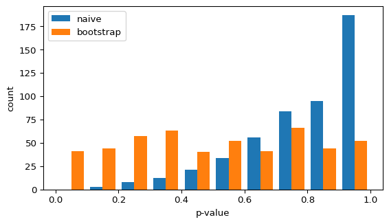
A valid test at level 5 % rejects 5 % of truly normal samples. Check both versions on 500 normal samples of size 200. The null distribution of $D$ is the same for all of them, so you simulate it once.

rng = np.random.default_rng(7)
m = 200
d_null = np.array([ks_stat_normal(rng.standard_normal(m)) for _ in range(1000)])
p_naive, p_boot = [], []
for _ in range(500):
    x = rng.normal(3.0, 2.0, m)
    d = ks_stat_normal(x)
    p_naive.append(stats.kstest(x, "norm", args=(x.mean(), x.std(ddof=1))).pvalue)
    p_boot.append((1 + np.sum(d_null >= d)) / (d_null.size + 1))
p_naive, p_boot = np.array(p_naive), np.array(p_boot)

fig, ax = plt.subplots(figsize=(6, 3.5))
ax.hist([p_naive, p_boot], bins=10, range=(0, 1), label=["naive", "bootstrap"])
ax.set_xlabel("p-value")
ax.set_ylabel("count")
ax.legend()
plt.tight_layout()
plt.show()
print(f"rejection rate at 5%: naive {np.mean(p_naive < 0.05):.3f}, bootstrap {np.mean(p_boot < 0.05):.3f}")

Figure 1: p-values of the naive KS test (parameters estimated, standard p-value) and of the bootstrap-calibrated test on 500 samples that really are normal. A valid test gives uniformly distributed p-values.

rejection rate at 5%: naive 0.000, bootstrap 0.048

The naive p-values pile up near 1 and almost never fall below 0.05. The bootstrap version rejects close to 5 % of the time, as it should.

Interpretation

The Q-Q plot, the Jarque-Bera test and the KS test ask the same question: are the returns consistent with an i.i.d. normal sample? For market data the answer is usually a clear no, because of the heavy tails you see in the Q-Q plot (cont2001empirical?).

Limitations

Every test here assumes i.i.d. data. Returns with volatility clustering are not i.i.d., so the bootstrap null distribution is only approximate.
With thousands of observations any test rejects even small departures from normality. Rejection says nothing about whether the departure matters for your purpose.
The Jarque-Bera test depends on moments that may not exist for heavy tails.

Optional extension

Exercise

Fit a Student-t distribution to the returns with stats.t.fit(r) and adapt the bootstrap KS test to it. The t family has a shape parameter, so the null distribution now depends on it: simulate from the fitted t and refit all three parameters on every bootstrap sample. Keep n_boot small (about 100) because stats.t.fit is slow.

Solution

The structure is the same as for the normal. Only the fit and the simulation change. A large p-value means the fitted t is consistent with the data at the level of the KS test. It does not remove the i.i.d. assumption.

def ks_stat_t(x):
    """KS distance between x and the Student-t fitted to x."""
    params = stats.t.fit(x)
    return stats.kstest(x, "t", args=params).statistic, params


def ks_t_bootstrap(x, n_boot, rng):
    d_obs, params = ks_stat_t(x)
    d_boot = np.array([
        ks_stat_t(stats.t.rvs(*params, size=x.size, random_state=rng))[0]
        for _ in range(n_boot)
    ])
    return d_obs, params, (1 + np.sum(d_boot >= d_obs)) / (n_boot + 1)


d_t, params_t, p_t = ks_t_bootstrap(r, n_boot=100, rng=np.random.default_rng(19))
print(f"fitted nu = {params_t[0]:.2f}; D = {d_t:.4f}; bootstrap p = {p_t:.3f}")

--- title: "Calibrated KS Test" subtitle: "Module 3: Modelling with Randomness" format: html --- The Kolmogorov-Smirnov (KS) test compares a whole distribution function with a model. Used naively with estimated parameters it gives wrong p-values. On this page you see why and build a version calibrated by simulation. You continue from [Normality Tests](normality-tests.qmd). ```{python} import matplotlib.pyplot as plt import numpy as np from scipy import stats from amlab.finance import load_prices, log_returns r = log_returns(load_prices()["close"]) ``` ## Why the plain KS test is not valid here The KS statistic is the largest distance between the empirical CDF $F_n$ and a model CDF $F$: $$ D = \sup_x |F_n(x) - F(x)| . $$ Kolmogorov's null distribution of $D$, which `scipy.stats.kstest` uses for its p-value, assumes that $F$ is fixed **before** you see the data. Here you do not know $\mu$ and $\sigma$; you estimate them from the same returns. The fitted normal is then pulled towards the data, so $D$ is systematically smaller than under a fixed $F$. The standard p-values are too large and the test rejects too rarely [@lilliefors1967kolmogorov]. @lilliefors1967kolmogorov obtained the correct null distribution by Monte Carlo. The same idea is a parametric bootstrap [@efron1979bootstrap]: simulate many normal samples of size $n$, estimate $\mu$ and $\sigma$ on each one, recompute $D$, and compare the observed $D$ with that simulated distribution. Because the normal is a location-scale family, the null distribution of $D$ with estimated parameters does not depend on the true $\mu$ and $\sigma$, so you can simulate from $\mathcal{N}(0, 1)$. ## Core activity: a bootstrap-calibrated KS test ::: {.callout-note} ## Exercise Complete the two functions. Then apply `ks_normal_bootstrap` to the returns with 300 bootstrap samples and compare its p-value with the naive one from `stats.kstest`. ```python def ks_stat_normal(x): """KS distance between x and the normal fitted to x.""" # TODO: estimate mu and sigma (ddof=1) and call stats.kstest(x, "norm", args=(mu, sigma)) return ... def ks_normal_bootstrap(x, n_boot, rng): d_obs = ks_stat_normal(x) # TODO: for n_boot repetitions, draw a standard normal sample of len(x) # and store ks_stat_normal of it d_boot = ... # TODO: p-value = (1 + number of d_boot >= d_obs) / (n_boot + 1) return d_obs, ... ``` ::: ::: {.callout-tip collapse="true"} ## Solution ```{python} def ks_stat_normal(x): """KS distance between x and the normal fitted to x.""" return stats.kstest(x, "norm", args=(x.mean(), x.std(ddof=1))).statistic def ks_normal_bootstrap(x, n_boot, rng): d_obs = ks_stat_normal(x) d_boot = np.array([ks_stat_normal(rng.standard_normal(x.size)) for _ in range(n_boot)]) return d_obs, (1 + np.sum(d_boot >= d_obs)) / (n_boot + 1) rng = np.random.default_rng(18) d_obs, p_boot = ks_normal_bootstrap(r, n_boot=300, rng=rng) p_naive = stats.kstest(r, "norm", args=(r.mean(), r.std(ddof=1))).pvalue print(f"D = {d_obs:.4f}; naive p = {p_naive:.2e}; bootstrap p = {p_boot:.4f}") ``` With 300 bootstrap samples the smallest possible p-value is $1/301 \approx 0.003$. A result at that floor means "smaller than 0.003". When the departure from normality is this large, both versions reject; the validation below shows where they differ. The function is also available as `amlab.finance.ks_normal_bootstrap`. ::: ## Validation: the test on data that are normal A valid test at level 5 % rejects 5 % of truly normal samples. Check both versions on 500 normal samples of size 200. The null distribution of $D$ is the same for all of them, so you simulate it once. ```{python} #| label: fig-lab-ks-validation #| fig-cap: "p-values of the naive KS test (parameters estimated, standard p-value) and of the bootstrap-calibrated test on 500 samples that really are normal. A valid test gives uniformly distributed p-values." rng = np.random.default_rng(7) m = 200 d_null = np.array([ks_stat_normal(rng.standard_normal(m)) for _ in range(1000)]) p_naive, p_boot = [], [] for _ in range(500): x = rng.normal(3.0, 2.0, m) d = ks_stat_normal(x) p_naive.append(stats.kstest(x, "norm", args=(x.mean(), x.std(ddof=1))).pvalue) p_boot.append((1 + np.sum(d_null >= d)) / (d_null.size + 1)) p_naive, p_boot = np.array(p_naive), np.array(p_boot) fig, ax = plt.subplots(figsize=(6, 3.5)) ax.hist([p_naive, p_boot], bins=10, range=(0, 1), label=["naive", "bootstrap"]) ax.set_xlabel("p-value") ax.set_ylabel("count") ax.legend() plt.tight_layout() plt.show() print(f"rejection rate at 5%: naive {np.mean(p_naive < 0.05):.3f}, bootstrap {np.mean(p_boot < 0.05):.3f}") ``` The naive p-values pile up near 1 and almost never fall below 0.05. The bootstrap version rejects close to 5 % of the time, as it should. ## Interpretation The Q-Q plot, the Jarque-Bera test and the KS test ask the same question: are the returns consistent with an i.i.d. normal sample? For market data the answer is usually a clear no, because of the heavy tails you see in the Q-Q plot [@cont2001empirical]. ## Limitations - Every test here assumes i.i.d. data. Returns with volatility clustering are not i.i.d., so the bootstrap null distribution is only approximate. - With thousands of observations any test rejects even small departures from normality. Rejection says nothing about whether the departure matters for your purpose. - The Jarque-Bera test depends on moments that may not exist for heavy tails. ## Optional extension ::: {.callout-note} ## Exercise Fit a Student-t distribution to the returns with `stats.t.fit(r)` and adapt the bootstrap KS test to it. The t family has a shape parameter, so the null distribution now depends on it: simulate from the fitted t and refit all three parameters on every bootstrap sample. Keep `n_boot` small (about 100) because `stats.t.fit` is slow. ::: ::: {.callout-tip collapse="true"} ## Solution The structure is the same as for the normal. Only the fit and the simulation change. A large p-value means the fitted t is consistent with the data at the level of the KS test. It does not remove the i.i.d. assumption. ```python def ks_stat_t(x): """KS distance between x and the Student-t fitted to x.""" params = stats.t.fit(x) return stats.kstest(x, "t", args=params).statistic, params def ks_t_bootstrap(x, n_boot, rng): d_obs, params = ks_stat_t(x) d_boot = np.array([ ks_stat_t(stats.t.rvs(*params, size=x.size, random_state=rng))[0] for _ in range(n_boot) ]) return d_obs, params, (1 + np.sum(d_boot >= d_obs)) / (n_boot + 1) d_t, params_t, p_t = ks_t_bootstrap(r, n_boot=100, rng=np.random.default_rng(19)) print(f"fitted nu = {params_t[0]:.2f}; D = {d_t:.4f}; bootstrap p = {p_t:.3f}") ``` :::