Traffic Model
Module 6: Explorables and Discrete Models
Traffic flow is a natural agent-based model. Each car moves according to simple local rules, but repeated interactions create stop-and-go waves, jams, and a transition between free flow and congestion (Nagel and Schreckenberg 1992). The rules are on the page The Nagel-Schreckenberg Model. In this lab you implement them.
Core activity
Implement step() for the Nagel-Schreckenberg model on a periodic road, validate it, and produce space-time diagrams for a free-flow and a congested density.
Prediction
Exercise
With \(v_{\max} = 5\) and \(p = 0\), below which density should every car end up moving at \(v_{\max}\)? What changes in the space-time diagram when you switch on \(p = 0.3\)?
Solution
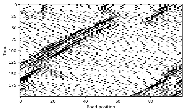
A car at \(v_{\max} = 5\) needs 5 empty cells ahead, so each car uses 6 cells. Below \(\rho = 1/(v_{\max}+1) = 1/6 \approx 0.17\) there is room for every car, and with \(p = 0\) all cars reach \(v_{\max}\) after a transient. With \(p = 0.3\) random slowdowns start jams even below that density. In the diagram they appear as dense, nearly horizontal bands that drift to the left, against the traffic.
What you need
numpystores the occupancy pattern, the speed of each car and the experimental results.matplotlib.pyplotplots space-time diagrams and flow-density curves.
Scripts or notebooks?
Use a notebook for density sweeps, repeated trials and parameter scans. Use a script if you want a faster interactive visualization or plan to add widgets later.
Represent the road state
We store the system with two arrays of length length:
occupied[i]tells us whether cellicontains a car.speeds[i]stores the speed of that car, measured in cells per step.
This lets the road stay discrete while each agent still has its own internal state.
Initialize the agents
The initialization function samples an occupancy pattern and assigns a random speed to each occupied cell.
occupied, speeds = initialize_road(length=100, density=0.2, vmax=5)The density is
\[ \rho = \frac{\text{number of cars}}{\text{road length}}. \]
Implement one synchronous update
At each time step, every car follows the same four rules:
- Accelerate up to \(v_{\max}\).
- Brake so it does not collide with the next car.
- Slow down randomly with probability \(p_{\text{slow}}\).
- Move forward by its new speed.
The key point is that all cars update synchronously.
Exercise
Complete step(). It returns the new occupancy and speed arrays after one synchronous update of all cars on a periodic road.
def step(occupied, speeds, vmax=5, p_slow=0.3, rng=None):
    if rng is None:
        rng = np.random.default_rng()

    # TODO: accelerate
    # TODO: brake to avoid collisions
    # TODO: random slowdown
    # TODO: move cars
    return new_occupied, new_speeds
Hint
Work with the car positions positions = np.where(occupied)[0], which are sorted along the road. The gap of a car is the number of empty cells up to the next car, (next_pos - pos - 1) % length. The next car of the last car in the list is the first car, because the road is a ring. Write all new speeds first and move the cars only at the end, so that every car sees the old configuration.
Solution
def step(occupied, speeds, vmax=5, p_slow=0.3, rng=None):
    if rng is None:
        rng = np.random.default_rng()

    length = len(occupied)
    positions = np.where(occupied)[0]
    speeds_new = speeds.copy()

    speeds_new[positions] = np.minimum(speeds_new[positions] + 1, vmax)

    gaps = np.zeros_like(positions)
    for idx, pos in enumerate(positions):
        next_pos = positions[(idx + 1) % len(positions)]
        gaps[idx] = (next_pos - pos - 1) % length
    speeds_new[positions] = np.minimum(speeds_new[positions], gaps)

    slow_mask = rng.random(len(positions)) < p_slow
    speeds_new[positions[slow_mask]] = np.maximum(
        speeds_new[positions[slow_mask]] - 1, 0
    )

    new_occupied = np.zeros_like(occupied)
    new_speeds = np.zeros_like(speeds)
    new_positions = (positions + speeds_new[positions]) % length
    new_occupied[new_positions] = True
    new_speeds[new_positions] = speeds_new[positions]

    return new_occupied, new_speeds
Validation
Three checks catch most bugs:
- the number of cars stays constant;
- no two cars ever occupy the same cell (the occupancy array keeps the same number of
Trueentries); - for \(p = 0\) and density below \(1/(v_{\max}+1)\), every car reaches \(v_{\max}\) after a transient.
import numpy as np
from amlab.cellular_automata.traffic import initialize_road, step

rng = np.random.default_rng(0)
occupied, speeds = initialize_road(length=120, density=0.1, vmax=5, rng=rng)
n_cars = occupied.sum()
for t in range(200):
    occupied, speeds = step(occupied, speeds, vmax=5, p_slow=0.0, rng=rng)
    assert occupied.sum() == n_cars, "a car was lost or two cars collided"
print("Cars:", n_cars, "| speeds after 200 steps:", np.unique(speeds[occupied]))
Cars: 15 | speeds after 200 steps: [5]Simulate a full run
Wrap the update in a loop and save the occupancy pattern at every time step.
grid = simulate(steps=200, length=100, density=0.2, vmax=5, p_slow=0.3, seed=1)Plot the space-time diagram
plt.imshow(grid, cmap="binary", interpolation="nearest", aspect="auto")
plt.xlabel("Road position")
plt.ylabel("Time")
plt.show()
What the dark bands mean
In the diagram, black cells are occupied sites. When dense diagonal bands become nearly horizontal, cars are moving slowly and congestion is forming. When the pattern is sparse and diagonal, cars are advancing freely.
Interpretation
A jam is not imposed externally. It emerges from repeated local braking and stochastic slowdown. Jams in the diagram drift to the left while cars move to the right: the jam front moves against the traffic.
Limitations
- The road is a ring with one lane, identical cars and identical drivers.
- The cell-based loop over cars in
step()is slow for long roads. The vectorized version in amlab/cellular_automata/traffic_models.py stores only the car positions.
Full reference: amlab/cellular_automata/traffic.py.
Next
Nagel, Kai, and Michael Schreckenberg. 1992. “A Cellular Automaton Model for Freeway Traffic.” Journal de Physique I 2 (12): 2221–29. https://doi.org/10.1051/jp1:1992277.