Scaling of Returns in Data

Module 3: Modelling with Randomness

In Scaling of Returns you saw the prediction $p_{\Delta t}(0) \propto \Delta t^{-1/\alpha}$ and the result $\alpha \approx 1.4$ of (mantegna1995scaling?) for minute data. Here you aggregate daily returns over longer horizons and test how the distribution changes with $\Delta t$.

import matplotlib.pyplot as plt
import numpy as np
from scipy import stats

from amlab.finance import load_prices, log_returns

r = log_returns(load_prices()["close"])
r = r - r.mean()
horizons = np.array([1, 2, 5, 10, 20, 50, 100])

WARNING: data/finance/prices.csv not found. Using a SYNTHETIC GARCH(1,1) series with Student-t innovations (seed 2026). These are not market data. See data/finance/README.md.

Prediction

Exercise

For each model below, predict how the standard deviation of $r(\Delta t)$ and its excess kurtosis change with $\Delta t$:

i.i.d. Gaussian returns;
i.i.d. returns with finite variance but fat tails;
returns that are uncorrelated but show volatility clustering.

Solution

In all three cases the standard deviation grows as $\sqrt{\Delta t}$, because the variances of uncorrelated terms add. The kurtosis tells the models apart:

i.i.d. Gaussian: the excess kurtosis is 0 at every horizon.
i.i.d. with fat tails (finite fourth moment): it starts positive and falls as $K_1 / \Delta t$.
Volatility clustering: it starts positive and falls more slowly than $K_1 / \Delta t$, because days in a calm or a turbulent period are not independent.

Core activity: aggregate the returns

The log return over $\Delta t$ days is the sum of $\Delta t$ daily log returns. Use non-overlapping blocks, so that different aggregated returns do not share days.

Exercise

Complete aggregate_returns. Then compute the standard deviation, the excess kurtosis and the density at zero of $r(\Delta t)$ for every horizon in horizons.

def aggregate_returns(r, horizon):
    """Sum r over non-overlapping blocks of length horizon."""
    m = # TODO: number of complete blocks
    # TODO: reshape r[: m * horizon] to (m, horizon) and sum along axis 1
    return ...

Solution

def aggregate_returns(r, horizon):
    """Sum r over non-overlapping blocks of length horizon."""
    m = r.size // horizon
    return r[: m * horizon].reshape(m, horizon).sum(axis=1)


def p_zero(x):
    """Density at 0, estimated in a window of one tenth of the IQR."""
    q75, q25 = np.percentile(x, [75, 25])
    eps = 0.1 * (q75 - q25)
    return np.mean(np.abs(x) < eps / 2) / eps


def scaling_table(r):
    """Standard deviation, excess kurtosis and p(0) at every horizon."""
    rows = []
    for h in horizons:
        x = aggregate_returns(r, h)
        rows.append((x.std(), stats.kurtosis(x), p_zero(x)))
    return np.array(rows)


table = scaling_table(r)
for h, (sd, kurt, p0) in zip(horizons, table):
    print(f"dt = {h:3d}: blocks {r.size // h:5d}, std {sd:.4f}, kurtosis {kurt:6.2f}, p(0) {p0:7.2f}")

dt =   1: blocks  5000, std 0.0091, kurtosis  11.97, p(0)   59.46
dt =   2: blocks  2500, std 0.0127, kurtosis   8.86, p(0)   45.14
dt =   5: blocks  1000, std 0.0206, kurtosis   4.24, p(0)   24.77
dt =  10: blocks   500, std 0.0294, kurtosis   5.64, p(0)   16.92
dt =  20: blocks   250, std 0.0396, kurtosis   1.31, p(0)   12.45
dt =  50: blocks   100, std 0.0697, kurtosis   1.03, p(0)    6.05
dt = 100: blocks    50, std 0.0913, kurtosis  -0.58, p(0)    3.37

aggregate_returns is also available in amlab.finance.

Validation: a shuffled series

Shuffling the returns in time keeps their distribution and destroys all dependence. The shuffled series is i.i.d. with the same fat tails. For it, the standard deviation must grow as $\sqrt{\Delta t}$ and, when the fourth moment is finite, the excess kurtosis of a sum of $\Delta t$ i.i.d. terms is the one-day value divided by $\Delta t$.

rng = np.random.default_rng(32)
table_shuffled = scaling_table(rng.permutation(r))
slope_sd = np.polyfit(np.log(horizons), np.log(table_shuffled[:, 0]), 1)[0]
print(f"shuffled: slope of log std vs log dt = {slope_sd:.3f} (theory 0.5)")

shuffled: slope of log std vs log dt = 0.497 (theory 0.5)

Experiment: three scaling plots

fig, axes = plt.subplots(1, 3, figsize=(10, 3.5))
for tab, label, marker in [(table, "original", "o"), (table_shuffled, "shuffled", "s")]:
    axes[0].loglog(horizons, tab[:, 0], marker, label=label)
    axes[1].semilogx(horizons, tab[:, 1], marker, label=label)
    axes[2].loglog(horizons, tab[:, 2], marker, label=label)
axes[0].loglog(horizons, table[0, 0] * np.sqrt(horizons), "k-", lw=0.8)
axes[1].semilogx(horizons, table[0, 1] / horizons, "k-", lw=0.8)
axes[2].loglog(horizons, table[0, 2] / np.sqrt(horizons), "k-", lw=0.8)
axes[0].set_ylabel("std of $r(\\Delta t)$")
axes[1].set_ylabel("excess kurtosis")
axes[2].set_ylabel("$p_{\\Delta t}(0)$")
for ax in axes:
    ax.set_xlabel("$\\Delta t$ (days)")
axes[0].legend()
plt.tight_layout()
plt.show()

slope_p0 = np.polyfit(np.log(horizons), np.log(table[:, 2]), 1)[0]
print(f"p(0) slope, original data: {slope_p0:.3f}  ->  effective alpha = {-1 / slope_p0:.2f}")

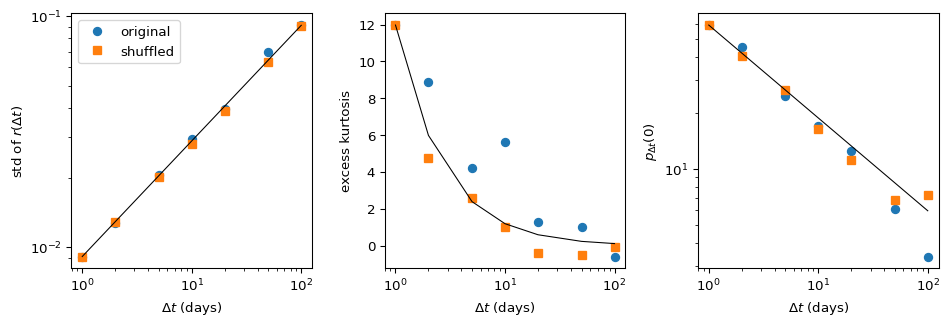
Figure 1: Scaling with the horizon $\Delta t$ for the original and the shuffled returns. Left: standard deviation, with slope 1/2. Centre: excess kurtosis, with the i.i.d. prediction $K_1/\Delta t$. Right: density at zero, with slope $-1/2$.

p(0) slope, original data: -0.616  ->  effective alpha = 1.62

Interpretation

The standard deviation grows close to $\sqrt{\Delta t}$ because daily returns are nearly uncorrelated. This is the part of the random walk model that survives.
The excess kurtosis falls with $\Delta t$: the distribution becomes more Gaussian at longer horizons, which is the aggregational Gaussianity of (cont2001empirical?). If it falls more slowly for the original data than for the shuffled data, the difference comes from volatility clustering, since that is the only thing the shuffle removed.
The effective $\alpha$ from $p_{\Delta t}(0)$ tells you whether the centre of the distribution rescales like a Lévy law or like a Gaussian over these horizons. (mantegna1995scaling?) found $\alpha \approx 1.4$ for horizons of 1 to 1000 minutes on the S&P 500; daily and longer horizons are a different regime.

Limitations

At $\Delta t = 100$ days a 20-year series gives only about 50 blocks. The kurtosis and $p(0)$ at long horizons are very noisy. Report them with that caveat or use overlapping blocks and account for the dependence they introduce.
The sample kurtosis is unreliable for heavy tails (cont2001empirical?). Use it to compare series, not as a precise value.
The $p(0)$ estimate depends on the window width. Try a few widths and check that your conclusion does not change.

Optional extension

Exercise

Plot the histograms of $r(\Delta t)/\Delta t^{1/2}$ for $\Delta t = 1, 5, 20$ on one log-density axis. If the returns scaled like a Gaussian random walk, the curves would collapse onto one. Repeat with $\Delta t^{1/1.4}$ and compare which rescaling collapses the centre better, as in (mantegna1995scaling?).

Solution

Loop over the two exponents and draw one panel for each. Judge the collapse near zero, not in the tails, where the long horizons have few points.

fig, axes = plt.subplots(1, 2, figsize=(9, 3.5), sharey=True)
for ax, alpha in zip(axes, [2.0, 1.4]):
    for h in [1, 5, 20]:
        x = aggregate_returns(r, h) / h ** (1 / alpha)
        dens, edges = np.histogram(x, bins=40, density=True)
        ax.semilogy(0.5 * (edges[1:] + edges[:-1]), dens, ".-", label=f"dt = {h}")
    ax.set_title(f"rescaled by dt^(1/{alpha})")
    ax.set_xlabel("rescaled return")
axes[0].set_ylabel("density")
axes[0].legend()
plt.tight_layout()
plt.show()

Exit question

Exercise

Suppose that on the same daily series the $p_{\Delta t}(0)$ method gives an effective $\alpha$ below 2 while the Hill estimator of Tail Exponent gives about 3. Is that a contradiction?

Solution

No. The two methods look at different parts of the distribution. The Hill estimator measures the far tail of one-day returns. The $p_{\Delta t}(0)$ method measures how the height of the centre changes under aggregation, which depends on the whole distribution and on the dependence between days. (mantegna1995scaling?) found exactly this combination for the S&P 500: a Lévy-like centre with $\alpha \approx 1.4$ and tails that fall off faster than a Lévy law, so the variance is finite. The truncated Lévy flight of (mantegna1994stochastic?) is one model with both properties.

--- title: "Scaling of Returns in Data" subtitle: "Module 3: Modelling with Randomness" format: html --- In [Scaling of Returns](scaling-of-returns.qmd) you saw the prediction $p_{\Delta t}(0) \propto \Delta t^{-1/\alpha}$ and the result $\alpha \approx 1.4$ of @mantegna1995scaling for minute data. Here you aggregate daily returns over longer horizons and test how the distribution changes with $\Delta t$. ```{python} import matplotlib.pyplot as plt import numpy as np from scipy import stats from amlab.finance import load_prices, log_returns r = log_returns(load_prices()["close"]) r = r - r.mean() horizons = np.array([1, 2, 5, 10, 20, 50, 100]) ``` ## Prediction ::: {.callout-note} ## Exercise For each model below, predict how the standard deviation of $r(\Delta t)$ and its excess kurtosis change with $\Delta t$: - i.i.d. Gaussian returns; - i.i.d. returns with finite variance but fat tails; - returns that are uncorrelated but show volatility clustering. ::: ::: {.callout-tip collapse="true"} ## Solution In all three cases the standard deviation grows as $\sqrt{\Delta t}$, because the variances of uncorrelated terms add. The kurtosis tells the models apart: - i.i.d. Gaussian: the excess kurtosis is 0 at every horizon. - i.i.d. with fat tails (finite fourth moment): it starts positive and falls as $K_1 / \Delta t$. - Volatility clustering: it starts positive and falls more slowly than $K_1 / \Delta t$, because days in a calm or a turbulent period are not independent. ::: ## Core activity: aggregate the returns The log return over $\Delta t$ days is the sum of $\Delta t$ daily log returns. Use non-overlapping blocks, so that different aggregated returns do not share days. ::: {.callout-note} ## Exercise Complete `aggregate_returns`. Then compute the standard deviation, the excess kurtosis and the density at zero of $r(\Delta t)$ for every horizon in `horizons`. ```python def aggregate_returns(r, horizon): """Sum r over non-overlapping blocks of length horizon.""" m = # TODO: number of complete blocks # TODO: reshape r[: m * horizon] to (m, horizon) and sum along axis 1 return ... ``` ::: ::: {.callout-tip collapse="true"} ## Solution ```{python} def aggregate_returns(r, horizon): """Sum r over non-overlapping blocks of length horizon.""" m = r.size // horizon return r[: m * horizon].reshape(m, horizon).sum(axis=1) def p_zero(x): """Density at 0, estimated in a window of one tenth of the IQR.""" q75, q25 = np.percentile(x, [75, 25]) eps = 0.1 * (q75 - q25) return np.mean(np.abs(x) < eps / 2) / eps def scaling_table(r): """Standard deviation, excess kurtosis and p(0) at every horizon.""" rows = [] for h in horizons: x = aggregate_returns(r, h) rows.append((x.std(), stats.kurtosis(x), p_zero(x))) return np.array(rows) table = scaling_table(r) for h, (sd, kurt, p0) in zip(horizons, table): print(f"dt = {h:3d}: blocks {r.size // h:5d}, std {sd:.4f}, kurtosis {kurt:6.2f}, p(0) {p0:7.2f}") ``` `aggregate_returns` is also available in `amlab.finance`. ::: ## Validation: a shuffled series Shuffling the returns in time keeps their distribution and destroys all dependence. The shuffled series is i.i.d. with the same fat tails. For it, the standard deviation must grow as $\sqrt{\Delta t}$ and, when the fourth moment is finite, the excess kurtosis of a sum of $\Delta t$ i.i.d. terms is the one-day value divided by $\Delta t$. ```{python} rng = np.random.default_rng(32) table_shuffled = scaling_table(rng.permutation(r)) slope_sd = np.polyfit(np.log(horizons), np.log(table_shuffled[:, 0]), 1)[0] print(f"shuffled: slope of log std vs log dt = {slope_sd:.3f} (theory 0.5)") ``` ## Experiment: three scaling plots ```{python} #| label: fig-lab-scaling #| fig-cap: "Scaling with the horizon $\\Delta t$ for the original and the shuffled returns. Left: standard deviation, with slope 1/2. Centre: excess kurtosis, with the i.i.d. prediction $K_1/\\Delta t$. Right: density at zero, with slope $-1/2$." fig, axes = plt.subplots(1, 3, figsize=(10, 3.5)) for tab, label, marker in [(table, "original", "o"), (table_shuffled, "shuffled", "s")]: axes[0].loglog(horizons, tab[:, 0], marker, label=label) axes[1].semilogx(horizons, tab[:, 1], marker, label=label) axes[2].loglog(horizons, tab[:, 2], marker, label=label) axes[0].loglog(horizons, table[0, 0] * np.sqrt(horizons), "k-", lw=0.8) axes[1].semilogx(horizons, table[0, 1] / horizons, "k-", lw=0.8) axes[2].loglog(horizons, table[0, 2] / np.sqrt(horizons), "k-", lw=0.8) axes[0].set_ylabel("std of $r(\\Delta t)$") axes[1].set_ylabel("excess kurtosis") axes[2].set_ylabel("$p_{\\Delta t}(0)$") for ax in axes: ax.set_xlabel("$\\Delta t$ (days)") axes[0].legend() plt.tight_layout() plt.show() slope_p0 = np.polyfit(np.log(horizons), np.log(table[:, 2]), 1)[0] print(f"p(0) slope, original data: {slope_p0:.3f} -> effective alpha = {-1 / slope_p0:.2f}") ``` ## Interpretation - The standard deviation grows close to $\sqrt{\Delta t}$ because daily returns are nearly uncorrelated. This is the part of the random walk model that survives. - The excess kurtosis falls with $\Delta t$: the distribution becomes more Gaussian at longer horizons, which is the aggregational Gaussianity of @cont2001empirical. If it falls more slowly for the original data than for the shuffled data, the difference comes from volatility clustering, since that is the only thing the shuffle removed. - The effective $\alpha$ from $p_{\Delta t}(0)$ tells you whether the centre of the distribution rescales like a Lévy law or like a Gaussian over these horizons. @mantegna1995scaling found $\alpha \approx 1.4$ for horizons of 1 to 1000 minutes on the S&P 500; daily and longer horizons are a different regime. ## Limitations - At $\Delta t = 100$ days a 20-year series gives only about 50 blocks. The kurtosis and $p(0)$ at long horizons are very noisy. Report them with that caveat or use overlapping blocks and account for the dependence they introduce. - The sample kurtosis is unreliable for heavy tails [@cont2001empirical]. Use it to compare series, not as a precise value. - The $p(0)$ estimate depends on the window width. Try a few widths and check that your conclusion does not change. ## Optional extension ::: {.callout-note} ## Exercise Plot the histograms of $r(\Delta t)/\Delta t^{1/2}$ for $\Delta t = 1, 5, 20$ on one log-density axis. If the returns scaled like a Gaussian random walk, the curves would collapse onto one. Repeat with $\Delta t^{1/1.4}$ and compare which rescaling collapses the centre better, as in @mantegna1995scaling. ::: ::: {.callout-tip collapse="true"} ## Solution Loop over the two exponents and draw one panel for each. Judge the collapse near zero, not in the tails, where the long horizons have few points. ```python fig, axes = plt.subplots(1, 2, figsize=(9, 3.5), sharey=True) for ax, alpha in zip(axes, [2.0, 1.4]): for h in [1, 5, 20]: x = aggregate_returns(r, h) / h ** (1 / alpha) dens, edges = np.histogram(x, bins=40, density=True) ax.semilogy(0.5 * (edges[1:] + edges[:-1]), dens, ".-", label=f"dt = {h}") ax.set_title(f"rescaled by dt^(1/{alpha})") ax.set_xlabel("rescaled return") axes[0].set_ylabel("density") axes[0].legend() plt.tight_layout() plt.show() ``` ::: ## Exit question ::: {.callout-note} ## Exercise Suppose that on the same daily series the $p_{\Delta t}(0)$ method gives an effective $\alpha$ below 2 while the Hill estimator of [Tail Exponent](tail-exponent.qmd) gives about 3. Is that a contradiction? ::: ::: {.callout-tip collapse="true"} ## Solution No. The two methods look at different parts of the distribution. The Hill estimator measures the far tail of one-day returns. The $p_{\Delta t}(0)$ method measures how the height of the centre changes under aggregation, which depends on the whole distribution and on the dependence between days. @mantegna1995scaling found exactly this combination for the S&P 500: a Lévy-like centre with $\alpha \approx 1.4$ and tails that fall off faster than a Lévy law, so the variance is finite. The truncated Lévy flight of @mantegna1994stochastic is one model with both properties. :::